For a long time now I have been looking for any proof that the MRB constant is special (better, greater, or otherwise different from what is usual) with no luck! Here is another such case in which I have found that all numbers are different; there exists signatures of numbers, like the biometrics of people! Numbers have telltales (etymology is "tell a tale" -- meaning "an outward sign" ) that we can use to identify them. The easiest telltale we all use is the digits of a number in a positive integer base. For example if a number starts out with "3.14159..,." that is a telltale that the number is probably pi, (at least we know it is in a close neighborhood)! In my search for justification of the MRB constant's existence, I began plotting the means of the decimal expansions of a few more well known numbers. By means, I say mean{(p}) = 1/Length[{p}] Sum[p[(1),p(2)p[(3)...], or average decimal value.
Here is our work::
First, because the MRB constant is not a standard constant in the Mathematica language, we need to quickly calculate a lot of digits of it:. From my beta version, for speed, of an old year 2012 program, they will be saved as MRBtest2: (This should take way less than 30 seconds, it takes my fast computer only 10 seconds.) Since this is a beta version, it has a few issues: if when you first rum it on a new local kernel, if a black-background widow pops up for a fraction of a second then abort the evaluation and run it over; it will run better now that the parallel kernels are activated!
Quiet[prec = 10000; ClearSystemCache[];
 T0 = SessionTime[];
 expM[pre_] :=
  Module[{a, d, s, k, bb, c, n, end, iprec, xvals, x, pc, cores = 16,
    tsize = 2^7, chunksize, start = 1, ll, ctab,
    pr = Floor[1.005*pre]}, chunksize = cores*tsize;
   n = Floor[1.32*pr];
   end = Ceiling[n/chunksize];
   Print["Iterations required: ", n];
   Print["end ", end]; Print[end*chunksize];
   d = (1/2)*(3 + 2*Sqrt[2])^n*(1 + (3 + 2*Sqrt[2])^(-2*n)); {b, c,
     s} = {SetPrecision[-1, 1.1*n], -d, 0}; iprec = Ceiling[pr/27];
   Do[xvals = Flatten[ParallelTable[Table[ll = start + j*tsize + l;
        x = N[ll^(1/ll), iprec]; pc = iprec;
        While[pc < pr, pc = Min[3*pc, pr]; x = SetPrecision[x, pc];
         y = x^ll - ll; x = x - (2*x*y)/(y + ll*(2*ll + y))];
        x, {l, 0, tsize - 1}], {j, 0, cores - 1},
       Method -> "EvaluationsPerKernel" -> 4]];
    ctab = ParallelTable[Table[c = b - c;
       ll = start + l - 2; b *= (2*(ll^2 - n^2))/(1 + 3*ll + 2*ll^2);
       c, {l, chunksize}], Method -> "EvaluationsPerKernel" -> 2];
    s += ctab.(xvals - 1); start += chunksize;
    Print["done iter ", k*chunksize, " ", SessionTime[] - T0];, {k, 0,
      end - 1}];
   N[-s/d, pr]]; t2 = Timing[MRBtest2 = expM[prec];];]
Here is a sample of what we will be doing:
First we will plot the values of the means of decimal expansions of MRBtest2:
ListPlot[Table[
  Total[Flatten[RealDigits[N[MRBtest2, u]]]]/u, {u, 10, 10000}]]
It is hard to say much about it, because we have nothing to compare it with.
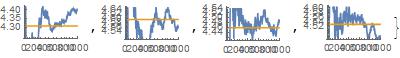
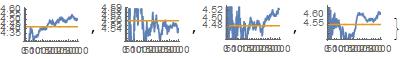
Let's plot some more well known constants with it: (I didn't put headings on our graphs when I first made them; I just went by the following convention when identifying them: The graphs are in the order given by the code as
1 2 3 4
or
1 2
3 4
const = {MRBtest2, E, EulerGamma, Sqrt[2]}; prec = 1000; aconst =
 N[const, prec]; Table[j = aconst[[z]];
 mp = Table[Total[Flatten[RealDigits[N[j, u]]]]/u, {u, 10, prec}];
 n = Table[Mean[mp], {x, 10, prec}]; ListLinePlot[{mp, n}], {z, 1, 4}]
Giving,
Now let's increase the desired precision and inspect the results in that dimension:
prec = 2000:
prec = 3000:
I will not post all the graphs from 4000 to 9000. We can do that separately.
Just, here are the graphs for
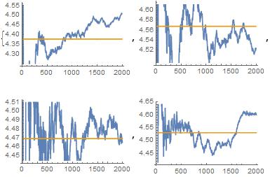
const = {MRBtest2, E, EulerGamma, Sqrt[2]}; prec = 10000; aconst =
 N[const, prec]; Table[j = aconst[[z]];
 mp = Table[Total[Flatten[RealDigits[N[j, u]]]]/u, {u, 10, prec}];
 n = Table[Mean[mp], {x, 10, prec}]; ListLinePlot[{mp, n}], {z, 1, 4}]
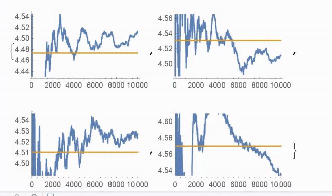
Notice that each graph has both subtle and profound differences from the others!!! In this case the differences are mostly profound!
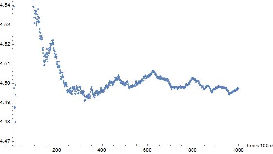
We don't want to make Hasty generalization of the future outcome (prec= O 10^m, m>10) because large numbers can have different results on the graphs of these functions than small numbers had! For example look at the SQRT{2] graph (the last graph in each set): It looks like it is headed new minimum, but further expansion gives the following dialog, which shows that we are only looking at a very minor part of a general negative value of the slope at most points:Understand that 4.54 is at the bottom of the last sqrt[2] graph shown above and at the top of the expanded graph below!!!
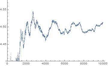
Warning! below we to save 100 fold time we will scale the x-axis and let n=10,000 be at x=100.
 ListPlot[Table[
   Total[Flatten[RealDigits[N[Sqrt[2], u]]]]/u, {u, 10, 100000, 100}]]
It was %3, then added
     Show[%3, AxesLabel -> {HoldForm[times 100 u], None},
      PlotLabel -> None, LabelStyle -> {GrayLevel[0]}]
I want to go know; I've been working on this for 9 hours straight now and FHV is on!
Look at, and further expand those graphs and see if there is anything you can say about the constants from the graphs.
Please provide your input --I am looking for real, proven advice and just plain old speculation.
So please say something!
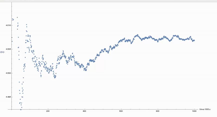
EDIT: Let's go a little further and see what happens to the mean of MRB constant expansions up to 1,000,000 digits, in steps of 1000: The million digits are from the over 3 million found in the file, 3M.nb, I uploaded into the original post of the lengthy and well read (probably not written!) discussion of
Try to beat these MRB constant records! . The 3 million+ digits took almost 2 months to compute using my fastest computer and a code similar to the one we got the above MRBtest2.
From.the following lines of code,
ListPlot[Table[
  Total[Flatten[RealDigits[N[MRBtest2, u]]]]/u, {u, 1000, 1000000,
   1000}]]
That became OUT[3], then we entered:
 Show[Out[57], AxesLabel -> {HoldForm[times 1000 u], None},
  PlotLabel -> None, LabelStyle -> {GrayLevel[0]}]
(Be warned again, the u value of 10,000 (we saw at the far right of the u axis in of the last of the MRB constant graphs) is now at x=10,probably only a fraction of a centimeter from the left onto the x-axis, below.)
The finished product is shown next: