Message Boards Message Boards

Graph a dual variable function?

Posted 9 years ago

I am trying to ListPlot the results of solving a quadratic in one variable as a function of a second variable. The equation is shown below:

((1-b)^2)*(R-r)^2=2*r*(1+b)^2,

where I am solving for r as a function of b. I can form the table, but it contains a mix of both branches of the solution to the quadratic equation in r. It is easy to solve but ListPlot will not plot the results. I am willing to live with the solution points mixed together, since the two branches will form two distinct curves and I can ignore the one that I cannot use.

Or, alternatively, how can I produce a graphic representation in some other way?

POSTED BY: Luther Nayhm
6 Replies

I would use

Manipulate[ContourPlot[(1 - b)^2*(R - r)^2 == 2*(1 + b)^2*r, {b, -1, 1}, {r, -5,5}], {R, 0.5, 2.0, 0.001}]

Then you can use the options in ContourPlot (ImageSize, PlotPoints, etc.) to make the display fit your needs. ContourPlot could be a bit slow (think of what it is doing), so each time you play with the value of R in the Manipulate scale you may need to wait a bit.

Best,

OL.

POSTED BY: Otto Linsuain
Posted 9 years ago

I see. Very nice. I have also played with the syntax and gotten a feel for the function I am plotting.

I appreciate the help. Thanks. I have a lot to learn about the minutia in using Mathematica.

POSTED BY: Luther Nayhm

[deleted double post]

POSTED BY: Jason Biggs
Posted 9 years ago

Clever. The documentation does not indicate what [All,1,2] means. Also the answer is given as (* *)...not sure I understand the meaning of these brackets and * symbols.

I wrote the function incorrectly. It needs two missing multiplication * symbols which I have inserted: Solve[((1 - b)^2)(R - r)^2 == 2r(1 + b)^2, r].....I occasionally forget the check the correct syntax and get funky answers that send me hunting. The one that is most confusing is following an exponent with another algebraic operation, like in the first term above: ((1-b)^2(R-r)^2...to bracket or not to bracket, that is the question.

The original equation that I solves is ((1-b)^2)/r^2=2*((1+b)^2)/(R-r)^2 which for a fixed value of R should solve for r with a finite range of values going to zero before b gets to unity. This model has a physical meaning and when b->1, it has one of those non-physical interpretations of something starting before it starts!!

The three dimensional plots are very nice...but R in the equation is a particular constant, so while it is nice to know what the 3D surface looks like, I am only using a single slice for the values I need.

All in all, thank you for the education.

POSTED BY: Luther Nayhm

In my post above, I put the output in comment markers - that is, anything between the (* and the *) are commented out.

So when you type the Solve command (note that you use two equal signs and not one, look at the help for Solve to see examples),

Solve[((1 - b)^2)/r^2 == 2*((1 + b)^2)/(R - r)^2, r]

this is the output,

{{r -> (-R + 2 b R - b^2 R - 
    Sqrt[2] Sqrt[R^2 - 2 b^2 R^2 + b^4 R^2])/(
   1 + 6 b + b^2)}, {r -> (-R + 2 b R - b^2 R + 
    Sqrt[2] Sqrt[R^2 - 2 b^2 R^2 + b^4 R^2])/(1 + 6 b + b^2)}}

This is in the form of a replacement rule ( type r^2 /. r->7 to see how a replacement rule works). But I wanted to grab the actual answers without copying and pasting them.

Here is another way to visualize your function:

define a function to be the solutions to the equations,

func[b_, R_] = 
  r /. Solve[((1 - b)^2)/r^2 == 2*((1 + b)^2)/(R - r)^2, r];
Plot[func[b, 1.0], {b, 0, 5}, Evaluated -> True]

enter image description here

These are the solutions for the equation when R=1.0, and you can plot them for any value of R.

POSTED BY: Jason Biggs

Here's how I would go about it,

solns = 
 Solve[((1 - b)^2) (R - r)^2 == 2 r*(1 + b)^2, r][[All, 1, 2]]
(* {(
 1 + 2 b + b^2 + R - 2 b R + b^2 R - Sqrt[
  1 + 4 b + 6 b^2 + 4 b^3 + b^4 + 2 R - 4 b^2 R + 2 b^4 R])/(
 1 - 2 b + b^2), (
 1 + 2 b + b^2 + R - 2 b R + b^2 R + Sqrt[
  1 + 4 b + 6 b^2 + 4 b^3 + b^4 + 2 R - 4 b^2 R + 2 b^4 R])/(
 1 - 2 b + b^2)} *)

You have to be careful as there is a singularity in the second solution when b=1:

Limit[#, b -> 1] & /@ solns
(* {0, ?} *)

So you can plot the first solution over any range,

Plot3D[solns[[1]], {b, 0, 10}, {R, 0, 10}, PlotRange -> All, 
 ColorFunction -> "ThermometerColors"]
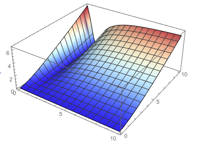
enter image description here

But the second solution you are limited in the range

Plot3D[solns[[2]], {b, 0, 5}, {R, 0, 10}, PlotPoints -> 100, 
 PlotRange -> {0, 50}, ColorFunction -> "ThermometerColors"]
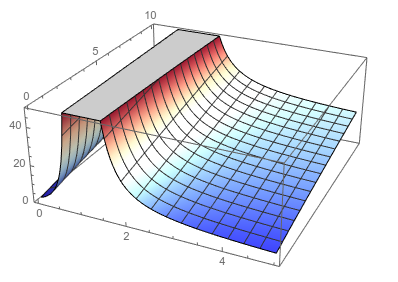
enter image description here

POSTED BY: Jason Biggs
Reply to this discussion
Community posts can be styled and formatted using the Markdown syntax.
Reply Preview
Attachments
Remove
or Discard

Group Abstract Group Abstract