Message Boards Message Boards

Graph a dual variable function?

Posted 9 years ago
POSTED BY: Luther Nayhm
6 Replies

I would use

Manipulate[ContourPlot[(1 - b)^2*(R - r)^2 == 2*(1 + b)^2*r, {b, -1, 1}, {r, -5,5}], {R, 0.5, 2.0, 0.001}]

Then you can use the options in ContourPlot (ImageSize, PlotPoints, etc.) to make the display fit your needs. ContourPlot could be a bit slow (think of what it is doing), so each time you play with the value of R in the Manipulate scale you may need to wait a bit.

Best,

OL.

POSTED BY: Otto Linsuain
Posted 9 years ago

I see. Very nice. I have also played with the syntax and gotten a feel for the function I am plotting.

I appreciate the help. Thanks. I have a lot to learn about the minutia in using Mathematica.

POSTED BY: Luther Nayhm

[deleted double post]

POSTED BY: Jason Biggs
Posted 9 years ago
POSTED BY: Luther Nayhm

In my post above, I put the output in comment markers - that is, anything between the (* and the *) are commented out.

So when you type the Solve command (note that you use two equal signs and not one, look at the help for Solve to see examples),

Solve[((1 - b)^2)/r^2 == 2*((1 + b)^2)/(R - r)^2, r]

this is the output,

{{r -> (-R + 2 b R - b^2 R - 
    Sqrt[2] Sqrt[R^2 - 2 b^2 R^2 + b^4 R^2])/(
   1 + 6 b + b^2)}, {r -> (-R + 2 b R - b^2 R + 
    Sqrt[2] Sqrt[R^2 - 2 b^2 R^2 + b^4 R^2])/(1 + 6 b + b^2)}}

This is in the form of a replacement rule ( type r^2 /. r->7 to see how a replacement rule works). But I wanted to grab the actual answers without copying and pasting them.

Here is another way to visualize your function:

define a function to be the solutions to the equations,

func[b_, R_] = 
  r /. Solve[((1 - b)^2)/r^2 == 2*((1 + b)^2)/(R - r)^2, r];
Plot[func[b, 1.0], {b, 0, 5}, Evaluated -> True]

enter image description here

These are the solutions for the equation when R=1.0, and you can plot them for any value of R.

POSTED BY: Jason Biggs

Here's how I would go about it,

solns = 
 Solve[((1 - b)^2) (R - r)^2 == 2 r*(1 + b)^2, r][[All, 1, 2]]
(* {(
 1 + 2 b + b^2 + R - 2 b R + b^2 R - Sqrt[
  1 + 4 b + 6 b^2 + 4 b^3 + b^4 + 2 R - 4 b^2 R + 2 b^4 R])/(
 1 - 2 b + b^2), (
 1 + 2 b + b^2 + R - 2 b R + b^2 R + Sqrt[
  1 + 4 b + 6 b^2 + 4 b^3 + b^4 + 2 R - 4 b^2 R + 2 b^4 R])/(
 1 - 2 b + b^2)} *)

You have to be careful as there is a singularity in the second solution when b=1:

Limit[#, b -> 1] & /@ solns
(* {0, ?} *)

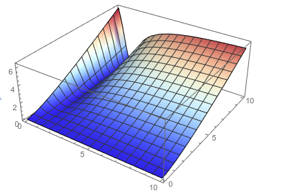
So you can plot the first solution over any range,

Plot3D[solns[[1]], {b, 0, 10}, {R, 0, 10}, PlotRange -> All, 
 ColorFunction -> "ThermometerColors"]

enter image description here

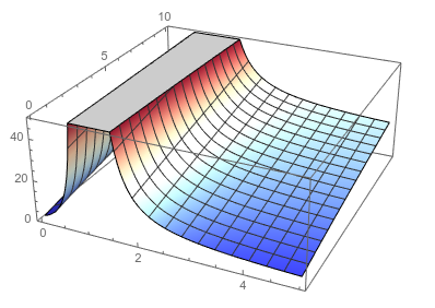
But the second solution you are limited in the range

Plot3D[solns[[2]], {b, 0, 5}, {R, 0, 10}, PlotPoints -> 100, 
 PlotRange -> {0, 50}, ColorFunction -> "ThermometerColors"]

enter image description here

POSTED BY: Jason Biggs
Reply to this discussion
Community posts can be styled and formatted using the Markdown syntax.
Reply Preview
Attachments
Remove
or Discard

Group Abstract Group Abstract