A chaotic system is one in which infinitesimal differences in the starting conditions lead to drastically different results as the system evolves.

Summarized by mathematician Edward Lorenz, "Chaos [is] when the present determines the future, but the approximate present does not approximately determine the future.“

There’s an important distinction to make between a chaotic system and a random system. Given the starting conditions, a chaotic system is entirely deterministic. A random system, on the other hand, is entirely non-deterministic, even when the starting conditions are known. That is, with enough information, the evolution of a chaotic system is entirely predictable, but in a random system there’s no amount of information that would be enough to predict the system’s evolution.

The simulations above show two slightly different initial conditions for a double pendulum — an example of a chaotic system. In the left animation both pendulums begin horizontally, and in the right animation the red pendulum begins horizontally and the blue is rotated by 0.1 radians (? 5.73°) above the positive x-axis. In both simulations, all of the pendulums begin from rest.

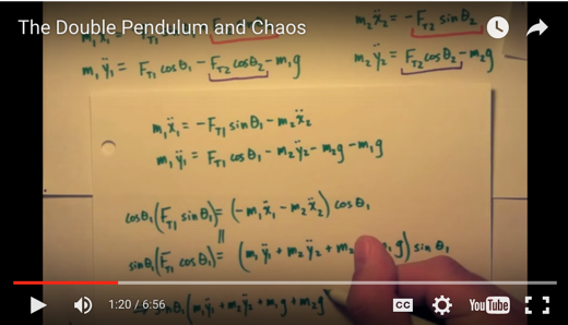
For more information on how to solve for the motion of a double pendulum, check out my video and Wolfram Language code below.

Originally published on Fouriest Series

x1[t_] := R1*Sin[?1[t]]
y1[t_] := (-R1)*Cos[?1[t]]
x2[t_] := R1*Sin[?1[t]] + R2*Sin[?2[t]]
y2[t_] := (-R1)*Cos[?1[t]] - R2*Cos[?2[t]]
v1[t_] := Sqrt[D[x1[t], t]^2 + D[y1[t], t]^2]
v2[t_] := Sqrt[D[x2[t], t]^2 + D[y2[t], t]^2]

T1[t_] := (1/2)*m1*v1[t]^2
T2[t_] := (1/2)*m2*v2[t]^2
U[t_] := m1*g*y1[t] + m2*g*y2[t]
L[t_] := T1[t] + T2[t] - U[t]

Simplify[D[LB[t], ?1B[t]] == D[D[LB[t], Derivative[1][?1B][t]], t]]; 
Simplify[D[LB[t], ?2B[t]] == D[D[LB[t], Derivative[1][?2B][t]], t]]; 

?10 = Pi/2; 
?1d0 = 0; 
?20 = Pi/2; 
?2d0 = 0; 

g = 9.8; 
R1 = 0.7; 
R2 = 0.7; 
m1 = 1; 
m2 = 1; 

sols = 
  NDSolve[
   {R1*(g*m1*Sin[?1[t]] + g*m2*Sin[?1[t]] + 
     m2*R2*Sin[?1[t] - ?2[t]]*Derivative[1][?2][t]^2 + 
     (m1 + m2)*R1*Derivative[2][?1][t] + 
     m2*R2*Cos[?1[t] - ?2[t]]*Derivative[2][?2][t]) == 0, 
    m2*R2*(g*Sin[?2[t]] - R1*Sin[?1[t] - 
      ?2[t]]*Derivative[1][?1][t]^2 + R1*Cos[?1[t] - 
      ?2[t]]*Derivative[2][?1][t] + R2*Derivative[2][?2][t]) == 0, 
    ?1[0] == ?10, 
    Derivative[1][?1][0] == ?1d0, 
    ?2[0] == ?20, 
    Derivative[1][?2][0] == ?2d0
   }, 
   {?1, Derivative[1][?1], Derivative[2][?1], 
    ?2, Derivative[1][?2], Derivative[2][?2]
   }, 
   {t, 0, 490}, 
   MaxSteps -> 100000
  ]; 

?1n[t_] := Evaluate[?1[t] /. sols[[1,1]]]
?2n[t_] := Evaluate[?2[t] /. sols[[1,4]]]
?d1n[t_] := Evaluate[Derivative[1][?1][t] /. sols[[1,1]]]
?d2n[t_] := Evaluate[Derivative[1][?2][t] /. sols[[1,4]]]

x1n[t_] := R1*Sin[?1n[t]]
y1n[t_] := (-R1)*Cos[?1n[t]]
x2n[t_] := R1*Sin[?1n[t]] + R2*Sin[?2n[t]]
y2n[t_] := (-R1)*Cos[?1n[t]] - R2*Cos[?2n[t]]

Manipulate[
  Show[
    ParametricPlot[
      {{x1n[t], y1n[t]}, {x2n[t], y2n[t]}}, 
      {t, 0, tf}, 
      PlotStyle -> {{Red}, {Blue}}, 
      AspectRatio -> Automatic, 
      PlotRange -> {{-R1 - R2, R1 + R2}, {-R1 - R2, (R1 + R2)/3.5}}, 
      Axes -> True, 
      GridLines -> Automatic, GridLinesStyle -> Directive[LightGray]
    ], 
    Graphics[
      {
        {AbsoluteThickness[2], Red, Line[{{0, 0}, {x1n[tf], y1n[tf]}}]}, 
        {AbsoluteThickness[2], Blue, Line[{{x1n[tf], y1n[tf]}, {x2n[tf], y2n[tf]}}]}, 
        {PointSize[Large], Red, Point[{x1n[tf], y1n[tf]}]}, 
        {PointSize[Large], Blue, Point[{x2n[tf], y2n[tf]}]}
      }
    ]
  ], 
  {tf, 0.01, 14, 0.1}
]