Introduction
A simplicial mesh is often used for the representation of surfaces. In the computational algorithm, typically it is more convenient to apply a piecewise linear mesh as the basis to formulate the problem like parametrization problems or simulation of the solution of partial differential equations. But in computational systems, it is not easy to use any mesh region. For instance, even in simply connected regions, a region without any hole inside, the boundary can be nowhere-differentiable and the computation can be highly complicated.
The Riemann mapping theorem guarantees a map from such a set in an angle-preserving manner to the regular unit disc. In 1985, Thurston posited that a regular circle packings may use for the approximation of the Riemannian map. In fact, circle packings assign a circle to each vertex of the mesh, with pairwise tangency for each edge in the mesh. Then try to find radii for these circles such that the combinatorially prescribed tangencies are maintained and the resulting arrangement of circles fills the desired region.
Thurston starts with a hexagonal circles packing, in which the radius of the circles creates a regular triangulated graph. Then he attaches all the boundary vertices to a point, let us say it is somewhere at infinity. After that he selects a face having one edge at the boundary and pulls all the other faces inside of the interstices of three boundary circles of the selected face and applies the circle packing algorithm. Finally, he removes the vertex infinity and inverts all the faces with respect to the circle centered at point infinity. In 1987, Rodin and Sullivan proved that Thurston's conjecture converges to the Riemann mapping. Although, Thurston's algorithm was based on hexagonal circle packing, in 2008 Shi-Yi Lana and Dao-Qing Dai generalized the convergence for the case of non-hexagonal cases.
In this project, we implement Thurston's algorithm for a non-hexagonal circle-packing to discretize conformal mappings.(A conformal mapping is an angle-preserving map between two spaces.) This result clearly shows the steps toward implementation of discretizing conformal map and it is very easy to understand and use even for the beginner in discrete geometry. Users only need to use the command RandomReal for n number points and select a face. For future work, one could try to optimize the code and compare it with the result in VaryLab which is specialized software for discrete surface optimization.
Outline
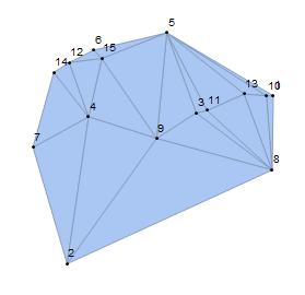
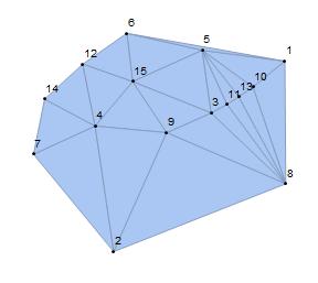
Step one: For a non-hexagonal circle pack, we use the RandomReal command for n points to create a Delaunay mesh. The output mesh assigns an irregular triangulated region. To identify the face f at the boundary, the user should run this part and select the face f in the order given by meshcell code. Note that since we are embedding all the faces inside of the face f, it is better to select a bigger face as f.
n = 15;
pts = RandomReal[1, {n, 2}];
delaunymesh = DelaunayMesh[pts];
meshcell = MeshCells[delaunymesh, 2];
infpts = n + 1;
f = {9, 2, 8};
HighlightMesh[
 DelaunayMesh[pts], {Style[0, Black], Labeled[0, "Index"]}]
Step Two:
According to Thurston's algorithm, boundary points are required for the mesh to attach them to the infinity point and then invert all the faces inside of the face f. The following code outputs a list of boundary edges and a list of inverted faces inside face f including faces created by attaching boundary points to the infinity point. We use counterclockwise order for the faces but it is possible to do it in the reverse order.
BoundaryEdgeList[delaunymesh_] :=
  Module[{meshcell, elist, x}, meshcell = MeshCells[delaunymesh, 2];
   elist = Part[meshcell, All, 1];
   Cases[GatherBy[Flatten[Partition[#, 2, 1, 1] & /@ elist, 1],
     Sort], {x_} :> x]];
Invertedfaces[delaunymesh_, bver_, f_, infpts_] :=
 Reverse /@
  Join[DeleteCases[Part[MeshCells[delaunymesh, 2], All, 1], f],
   Map[Reverse[#] &,
     Append[#, infpts] & /@ BoundaryEdgeList[delaunymesh]];
The following code computes the radii of the three boundary circles for the face f.
radi[d12_, d13_,
   d23_] := {(d12 + d13 - d23)/2, (d12 + d23 - d13)/
    2, (d23 + d13 - d12)/2};
Radif[f_, pts_] :=
  radi[EuclideanDistance[pts[[f]][[1]], pts[[f]][[2]]],
   EuclideanDistance[pts[[f]][[1]], pts[[f]][[3]]],
   EuclideanDistance[pts[[f]][[2]], pts[[f]][[3]]]];
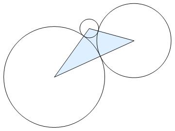
The command ThurstonAlg takes that data and assigns a circle to each vertex of the inverted faces with pairwise tangency for each edge of the faces. Then it evaluates the radii for those circles such that the combinatorially prescribed tangencies are maintained and the resulting arrangement of circles fills the interstices of the three boundary circles.
ThurstonsAlg[f1_, f_, radif_, maxsteps_: 250] :=
  Module[{vlist = Complement[Flatten[f1], f], x, ngbedges},
   ngbedges =
    Map[Function[v,
      v -> DeleteCases[Select[f1, MemberQ[#, v] &], v, 2]], vlist];
   FixedPoint[
    Join[MapThread[#1 -> #2 &, {f, radif}],
      Function[v,
        v -> (x /.
           FindRoot[
             2 Pi ==
              Plus @@
               Function[{y, z},
                 ArcCos[((x + y)^2 + (x + z)^2 - (y + z)^2)/(
                  2 (x + y) (x + z))]] @@@ (v /.
                   ngbedges /. #), {x, .6, 10^-10, 100}][[1]])] /@
       vlist] &, # -> 1 & /@ Union[Flatten[f1]], maxsteps]
   ];
Challenge:
To invert the circles packing, related to the circle centered at the point infinity, the coordinates of circles' center was required, which was the most difficult part of the work. Ultimately, we constituted a linear structure of the faces' edges, the g code, and tried to minimize them in the regional interstices of the three boundary circles by the command regionint.
g = Sum[((# - #2).(# - #2) &[Lookup[coordinates, FirstPoint[edge]],
       Lookup[coordinates, SecondPoint[edge]]] -
      Lookup[distanceassociation, List[edge]][[1]]^2)^2, {edge,
    alledges}];
r1 = RegionUnion[
   MapThread[
    Disk, {ptsf,
     radi[EuclideanDistance[ptsf[[1]], ptsf[[2]]],
      EuclideanDistance[ptsf[[1]], ptsf[[3]]],
      EuclideanDistance[ptsf[[2]], ptsf[[3]]]]}]];
r2 = Triangle[pts[[f]]];
regionint = DiscretizeRegion[RegionDifference[r2, r1]]
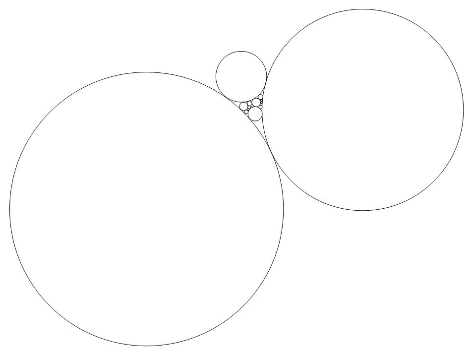
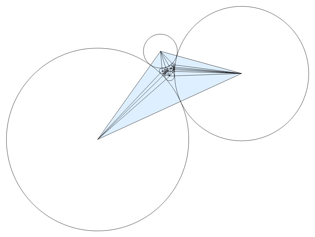
Graph bellow shows the minimized linear structure in the regional interstices of the three boundary circles and its circle packing.
Graphics[{LightBlue, Polygon[ptsf],
  Black, {MapThread[Circle, {CenterPoints, radii}],
   Line[(DeleteDuplicates[
       Map[Sort,
        Flatten[Map[Partition[#, 2, 1, 1] &, Part[f1, All]], 1]]]) /.
     Table[i -> CenterPoints[[i]], {i, 1, n + 1}]]}}]
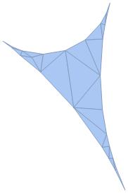
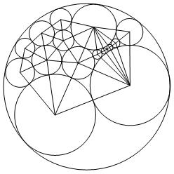
Lastly, to invert the new circles, related to the circle centered at the point infinity, we eliminated vertex infinity and applied the inversion formula. Invertcircles outputs the inverted coordinate of the circles' center and InvertRadii outputs inverted radii for each circle. The combination of this data results in an arrangement of the circles which fills the circle centered at the point infinity.
Invertcircles[v_, CenterPoints_,
   G_] := (radii[[
         v]]^2 (CenterPoints[[#1]] - CenterPoints[[v]]))/(Norm[
         CenterPoints[[#1]] - CenterPoints[[v]]]^2 - radii[[#1]]^2) +
     CenterPoints[[v]] & /@ G;
InvertRadii[v_, CenterPoints_, G_] :=
  #1 -> radii[[#1]] Abs[
       radii[[v]]^2/(Norm[CenterPoints[[#1]] - CenterPoints[[v]]]^2 -
          radii[[#1]]^2)] & /@ G;
Graphics[{MapThread[Circle, {Invertcircles, Values[InvertRadii]}],
  Circle[CenterPoints[[infpts]], radii[[infpts]]],
  Line[(DeleteDuplicates[
      Map[Sort,
       Flatten[Map[Partition[#, 2, 1, 1] &, Part[meshcell, All, 1]],
        1]]]) /. Table[i -> Invertcircles[[i]], {i, 1, n}]]}]
Acknowledgements:
This project was under the mentorship program supported by Wolfram Research Inc and I am highly indebted to them for their support. I would like to express my special gratitude and thanks to Dr, Todd Rowland, and Dr, Matthew Szudzik for their supervision and constant support in completing this project. My thanks and appreciations also go to Ms. Alison Kimball for her guidance and providing necessary information regarding this project.
Final code
radi[d12_, d13_,
   d23_] := {(d12 + d13 - d23)/2, (d12 + d23 - d13)/
    2, (d23 + d13 - d12)/2};
Radif[f_, pts_] : =
  radi[EuclideanDistance[pts[[f]][[1]], pts[[f]][[2]]],
   EuclideanDistance[pts[[f]][[1]], pts[[f]][[3]]],
   EuclideanDistance[pts[[f]][[2]], pts[[f]][[3]]]];
radif = Radif[f, pts];
BoundaryEdgeList[delaunymesh_] :=
  Module[{meshcell, elist, x}, meshcell = MeshCells[delaunymesh, 2];
   elist = Part[meshcell, All, 1];
   Cases[GatherBy[Flatten[Partition[#, 2, 1, 1] & /@ elist, 1],
     Sort], {x_} :> x]];
bver = BoundaryEdgeList[delaunymesh];
Invertedfaces[delaunymesh_, bver_, f_, infpts_] :=
  Reverse /@
   Join[DeleteCases[Part[MeshCells[delaunymesh, 2], All, 1], f],
    Map[Reverse[#] &, Append[#, infpts] & /@ bver]];
f1 = Invertedfaces[delaunymesh, bver, f, infpts];
ThurstonsAlg[f1_, f_, radif_, maxsteps_: 250] :=
  Module[{vlist = Complement[Flatten[f1], f], x, ngbedges},
   ngbedges =
    Map[Function[v,
      v -> DeleteCases[Select[f1, MemberQ[#, v] &], v, 2]], vlist];
   FixedPoint[
    Join[MapThread[#1 -> #2 &, {f, radif}],
      Function[v,
        v -> (x /.
           FindRoot[
             2 Pi ==
              Plus @@
               Function[{y, z},
                 ArcCos[((x + y)^2 + (x + z)^2 - (y + z)^2)/(
                  2 (x + y) (x + z))]] @@@ (v /.
                   ngbedges /. #), {x, .6, 10^-10, 100}][[1]])] /@
       vlist] &, # -> 1 & /@ Union[Flatten[f1]], maxsteps]
   ];
radii = ThurstonsAlg[f1, f, radif, 250];
Off[NMinimize::incst];
Off[NMinimize::nosat];
NewPointsLocation[f1_, radii_, f_, pts_, infpts_] :=
  Module[{alledges, ptsf, FirstPoint, SecondPoint,
    distanceassociation, knownpoints, coordinates, LeftQ, fd,
    constraints, variables, g, r1, r2, region},
   alledges =
    DeleteDuplicates[
     Map[Sort, Flatten[Map[Partition[#, 2, 1, 1] &, f1], 1]]];
   ptsf = pts[[f]];
   FirstPoint[{x_, y_}] := x;
   SecondPoint[{x_, y_}] := y;
   distanceassociation =
    Association[
     Table[edge ->
       radii[[FirstPoint[edge]]] + radii[[SecondPoint[edge]]], {edge,
       alledges}]];
   knownpoints =
    Flatten[{x[#] -> pts[[#, 1]], y[#] -> pts[[#, 2]]} & /@ f];
   coordinates =
    Association[
     Table[i -> {x[i], y[i]}, {i, 1, infpts}] /. knownpoints];
   variables = Cases[Values[coordinates], _x | _y, Infinity];
   g = Sum[((# - #2).(# - #2) &[Lookup[coordinates, FirstPoint[edge]],
          Lookup[coordinates, SecondPoint[edge]]] -
        Lookup[distanceassociation, List[edge]][[1]]^2)^2, {edge,
      alledges}];
   LeftQ[{a_, b_, c_}] := Det[{a - c, b - c}] > 0;
   fd = f1 /. coordinates;
   constraints = Apply[And, LeftQ[#] & /@ fd];
   r1 = RegionUnion[
     MapThread[
      Disk, {ptsf,
       radi[EuclideanDistance[ptsf[[1]], ptsf[[2]]],
        EuclideanDistance[ptsf[[1]], ptsf[[3]]],
        EuclideanDistance[ptsf[[2]], ptsf[[3]]]]}]];
   r2 = Triangle[pts[[f]]];
   region =
    Apply[And, {Element[#, RegionDifference[r2, r1]] & /@
       Partition[variables, 2]}];
   Minimize[{g, constraints}, region]];
CenterPoints = NewPointsLocation[f1, radii, f, pts, infpts];
CenterPoints =
  Values[Sort[
    Partition[
     Join[Flatten[{x[#] -> pts[[#, 1]], y[#] -> pts[[#, 2]]} & /@ f],
      Newpts[[2]]], 2]]];
Graphics[{LightBlue, Polygon[ptsf],
  Black, {MapThread[Circle, {CenterPoints, radii}],
   Line[(DeleteDuplicates[
       Map[Sort,
        Flatten[Map[Partition[#, 2, 1, 1] &, Part[f1, All]], 1]]]) /.
     Table[i -> CenterPoints[[i]], {i, 1, n + 1}]]}}]
G = Range[n];
v = infpts;
Invertcircles[v_, CenterPoints_,
   G_] := (radii[[
         v]]^2 (CenterPoints[[#1]] - CenterPoints[[v]]))/(Norm[
         CenterPoints[[#1]] - CenterPoints[[v]]]^2 - radii[[#1]]^2) +
     CenterPoints[[v]] & /@ G;
InvertRadii[v_, CenterPoints_, G_] :=
  #1 -> radii[[#1]] Abs[
       radii[[v]]^2/(Norm[CenterPoints[[#1]] - CenterPoints[[v]]]^2 -
          radii[[#1]]^2)] & /@ G;
Graphics[{MapThread[Circle, {Invertcircles, Values[InvertRadii]}],
  Circle[CenterPoints[[infpts]], radii[[infpts]]],
  Line[(DeleteDuplicates[
      Map[Sort,
       Flatten[Map[Partition[#, 2, 1, 1] &, Part[meshcell, All, 1]],
        1]]]) /. Table[i -> Invertcircles[[i]], {i, 1, n}]]}]


