The research project is concerned with the simulation and visualization of waves in three dimensional complex structures. In this project we use finite element analysis to investigative the propagation of elastic waves at the earth surface. The structure of the Geographic location is extracted from its map, meshed and used in the calculations. In addition we will be able to visualize the waves.
- Extraction of the geographical region.
- Simulation of the elastic waves.
- Visualization of the displacement vector field
Waves on the flat region
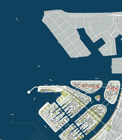
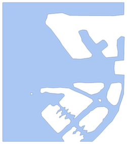
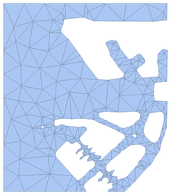
First we start with wave simulation on the flat surface in the region that can be created from an image using the new function ImageMesh. Here we imported the image longkouImg of the Longkou West Coast Artificial Island. Then we have created the Binarized image
longkouImgBinarized = ColorNegate@
   FillingTransform[
    Binarize[ColorConvert[
      GaussianFilter[longkouImg, 4], "Grayscale"], 0.6], 2];
ImageMesh can convert the binary image into Mathematica region
longkouRegion = ImageMesh[longkouImgBinarized ];

longkouRegion = RegionResize[
   longkouRegion, {{0,
     1}, {0, (Divide @@ ImageDimensions[longkouImg])^-1}}];
The mesh will have the following form
DiscretizeRegion[longkouRegion,
 MaxCellMeasure -> .01, AccuracyGoal -> 7]
Having the region, we define wave differential equation. And then solve them in the region with some initial conditions.
$$\frac{d^2 u(t,x,y)}{\text{dt}^2}-\nabla _{\{x,y\}}^{}u(t,x,y)=0 $$
uWavelongkou = NDSolveValue[{D[u[t,x,y] ,{t,2}]- Inactive[Laplacian][u[t, x, y], {x, y}] == 0,
                             u[0, x, y] == E^(-500(x - 0.2)^2 - 500(y - 0.8)^2),
                            (D[u[t, x, y],t]/. t->0 )== 0,
                             DirichletCondition[u[t, x, y] == 0, True]},
                             u, {t, 0,  1}, {x, y} \[Element] longkouRegion]

framesWEQ=Table[Plot3D[uWavelongkou[t,x,y],{x,y}\[Element]longkouRegion,SphericalRegion->True,
               PlotRange->All,PlotPoints->50,PlotStyle->Directive[LightBrown,Specularity[White,20],
               Opacity[0.9]],Boxed->False,Axes->None,Mesh->None],{t,0,1,0.1}]
3D case
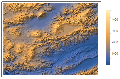
Now let's proceed to the 3D case. Here we mainly use GeoElevationData to get the elevations for geographical region. The plot of its relief shown below
ReliefPlot[
 GeoElevationData[GeoDisk[{40.7, 44.7}, Quantity[100, "Miles"]]],
 PlotLegends -> Automatic]
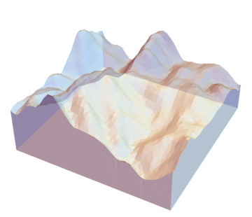
First, using geodesy and elevation data provided by Wolfram Language we modeled the environment were the propagation of wave will be simulated. The block geoRangeToRegion takes the range with geoPositions, then uses the GeoElevationData of the specified geo region to construct the interpolation function of the elevation. Than using that interpolation function we can construct implicit region.
geoRangeToRegion[loc1_, loc2_, detalization_, maxCell_,
minMaxHeight_] := Module[
{x, y, z, lat1, lat2, long1, long2, data, dataInter, xrange, yrange,
zrange, interpolation, reg},
{lat1, long1} = loc1;
{lat2, long2} = loc2;
data = Flatten[First@
GeoElevationData[{GeoPosition[{lat1, long1}],
GeoPosition[{lat2, long2}]},
"Geodetic", "GeoPosition", GeoZoomLevel -> detalization], 1];
data[[All, 1 ;; 2]] = (data[[All, 1 ;; 2]])*111.;
data[[All, 1 ;; 2]] = -loc1*111 + # & /@ data[[All, 1 ;; 2]];
data[[All, 3]] = data[[All, 3]]/1000;
xrange = MinMax@data[[All, 1]];
yrange = MinMax@data[[All, 2]];
zrange = MinMax@data[[All, 3]];
dataInter = {#[[1 ;; 2]], #[[3]]} & /@ data;
interpolation = Interpolation[dataInter];
reg = ImplicitRegion[
xrange[[1]] <= x <= xrange[[2]]
&& yrange[[1]] <= y <= yrange[[2]] &&
0 < z <= interpolation[x, y], {x, y, z}];
DiscretizeRegion[reg, {xrange, yrange, minMaxHeight},
MaxCellMeasure -> maxCell]
]
region = geoRangeToRegion[{40.7, 44.7}, {41, 45}, 7, 1, {0.5, 4}];
RegionPlot3D[region, BoxRatios -> {2, 2, 1},
PlotPoints -> 80, Boxed -> False,
PlotStyle -> Directive[LightBlue, Opacity[0.5]],
Axes -> False, AxesLabel -> {"x,km", "y,km", "z,km"},
LabelStyle -> Directive[Bold, Medium]]
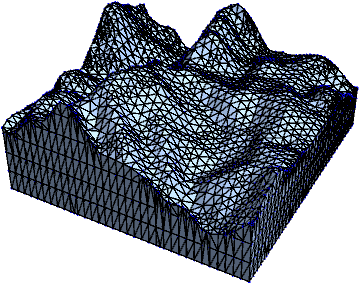
DiscretizeRegion[region,
MeshCellStyle -> {{1, All} -> Black, {0, All} -> Blue},
MaxCellMeasure -> 10, BoxRatios -> {2, 2, 1}, AccuracyGoal -> 5]
For 3D case of elasticity wave propagation we assume that the considered media is homogeneous and isotropic. The constitutive relation between stresses and strains for a homogeneous and isotropic material can be expressed by Hooke' s law. By definition, a homogeneous and isotropic material has the same properties in all directions. From this, the following equations for direct strain in terms of stress are presented
$$\sigma _{\text{ii}}=2 \mu \varepsilon _{\text{ii}}+\lambda \left(\varepsilon _{\text{xx}}+\varepsilon _{\text{yy}}+\varepsilon _{\text{zz}}\right)$$ $$\sigma _{\text{ij}}=2 \mu \varepsilon _{\text{ij}}$$
were $\mu$ and $\lambda$ are Lame's elastic constants, are the element of the strain tensor and $\sigma _{\text{ij}}$ the stress tensor. Combing this to equation of the motion. We arrive to Naiver Lame equations
$$(\lambda +\mu ) \text{Grad}\left[\nabla _{\{x,y,z\}}\cdot \overset{\rightharpoonup }{u}(t,x,y,z)\right]+\mu \text{Laplacian}\left[\overset{\rightharpoonup }{u}(t,x,y,z)\right]=\frac{d^2 \rho \overset{\rightharpoonup }{u}(t,x,y,z)}{\text{dt}^2}$$
ct = 1;
cl = 2;
Then the system of differential equations for the displacement components with initial and boundary conditions are below
uifWave = NDSolveValue[{D[ux[t,x,y,z] ,{t,2}]-(cl^2- ct^2) D[D[ ux[t,x,y,z],x]+D[uy[t,x,y,z],y]+D[uz[t,x,y,z],x],x]
                        -ct^2 Inactive[Laplacian][ux[t,x, y, z], {x,  y, z}] == 0,

                         D[uy[t,x,y,z] ,{t,2}] - (cl^2- ct^2) D[D[ ux[t,x,y,z],x]+D[uy[t,x,y,z],y] +D[uz[t,x,y,z],x],y]
                         -ct^2 Inactive[Laplacian][uy[t,x, y, z] , {x, y, z}] == 0,

                         D[uz[t,x,y,z] ,{t,2}] - (cl^2- ct^2) D[D[ ux[t,x,y,z],x]+D[uy[t,x,y,z],y] +D[uz[t,x,y,z],x],z]
                         -ct^2 Inactive[Laplacian][uz[t,x, y, z] , {x, y, z}] == 0,

                         ux[0,x, y,z]==(x - 15)E^(-0.1(x - 15)^2 - 0.1(y - 15)^2 -100(z - 0.6)^2),
                         uy[0,x, y,z]==0,
                         uz[0,x, y,z]==0,

                         (D[ux[t, x, y,z],t]/. t->0 )== 0,
                         (D[uy[t, x, y,z],t]/. t->0 )== 0,
                         (D[uz[t, x, y,z],t]/. t->0 )== 0,

                         DirichletCondition[ux[t,x, y, z] == 0, True],
                         DirichletCondition[uy[t,x, y, z] == 0, True],
                         DirichletCondition[uz[t,x, y, z] == 0, True]},

                        {ux,uy,uz}, {t, 0, 1}, {x, y,z} \[Element] regionoffline]


    lst = Table[Show[VectorPlot3D[{
          uifWave[[1]][t, x, y, z], uifWave[[2]][t, x, y, z],
          uifWave[[3]][t, x, y, z]},
         {x, 1.2, 30}, {y, 1.2, 30}, {z, 0.52, 2.5},
         PlotRange -> Automatic, VectorStyle -> Red, VectorPoints -> 10,
         VectorScale -> 0.05,
         RegionFunction ->
          Function[{x, y, z}, {x, y, z} \[Element] region]],
        RegionPlot3D[region,
         PlotStyle ->
          Directive[Blue, Opacity[0.2], PlotRange -> All,
           Boxed -> False]]], {t, 0, 1, 0.1}];