Introduction
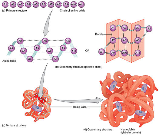
Proteins play crucial roles in the living cell and are involved in various vital processes. Protein sequences are not random, just as random sequences of letters and spaces rarely form words or sentences. Rather, protein sequences are "designed by evolution" i.e.the polypeptide chains, which did not fold in a biologically relevant time into a functional state and made the host organism less competitive, disappeared due to natural selection. Natural protein sequences are the result of many trials and errors. Important to notice that folding into specific structures in a biologically relevant time is a necessary but not a sufficient condition for an amino acid sequence to be a protein sequence.There is more information encrypted in protein sequences that needs to be understood. Our aim is to find out the regularities in the protein sequences that are absent in the randomly generated sequences of amino acids.
Results and discussion
- Data importation (transmembrane protein sequences)
- Sequence length statistics
- Sequence structure statistics
- Random amino acid sequence generation
- Random sequence structure statistics
- Guessing whether given sequence is a transmembrane protein sequence The code was also implemented for analyzing sequences of letters in English, German, Italian, Russian, Arabic and Hebrew words.
We decided to take sequences of the transmembrane proteins from the human protein data that is available in Mathematica 11.
(*Chose transmembrane proteins*)
(tr = {#, ProteinData[#, "Sequence"]} & /@
    Take[Select[ProteinData["Classes"],
      StringMatchQ[
        CanonicalName[#], ___ ~~ "Transmembrane" ~~ ___] &]]) // Short

(*Take sequences of transmembrane proteins*)
(trseq = DeleteCases[Flatten[tr], a_ /; StringQ[a] != True]) // Short
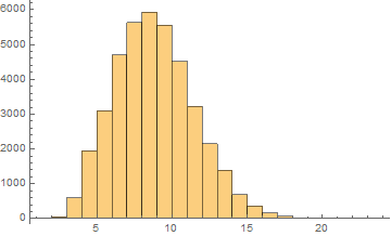
Next we did some basic statistical anayses of the sequence lengths.
Histogram[Map[Length, Characters[trseq]]]
Print[ "Mean sequence length = ",
 N[Mean[Map[Length, Characters[trseq]]]]]
Print["Median sequence length = ",
 N[Median[Map[Length, Characters[trseq]]]]]
Print["SD of the sequence lengths = ",
 N[StandardDeviation[Map[Length, Characters[trseq]]]]]
Print["Skewness of the sequence lengths = ",
 N[Skewness[Map[Length, Characters[trseq]]]]]
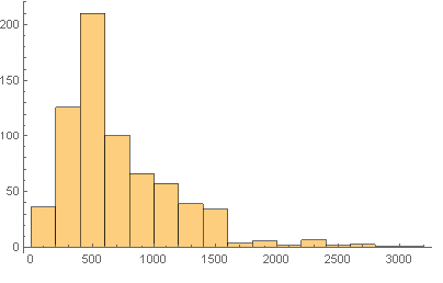
Mean sequence length = 714.987
Median sequence length = 559.
SD of the sequence lengths = 465.857
Skewness of the sequence lengths = 1.58423
In protein sequences there are evolutionary preserved regions that are important for some function, thus it is important to determine the sub-sequences that are frequently occurring in protein sequences. This was achieved through CharacterCounts function in Mathematica 11:
(*Finds the most frequently occurring subsequences.Probably those are
evolutionary preserved and hence are important parts of the
protein*)(*the computaion time takes around 1 min*)
tab = Table[
   Sort[Merge[CharacterCounts[Flatten[trseq], n], Total],
    Greater], {n, 1, 20, 1}];
Then it was visualized as a table and bar chart:
(*Generates a hierarchical table of most frequently occurring
subsequences of a given length.The length of the subsequence can vary
between 1 and 20*)
Manipulate[Dataset[Take[tab[[i]], {1, 20}]], {i, 1, 20, 1}]

(*Generates a hierarchical table of most frequently occurring
subsequences of a given length.The length of the subsequence can vary
between 1 and 20*)
Manipulate[
 BarChart[Take[tab[[i]], {1, 20}],
  ChartLabels ->
   Placed[ToString /@ Automatic, Axis, Rotate[#, Pi/2] &]], {i, 1, 20,
   1}]
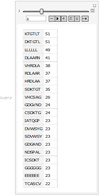
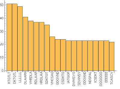
From the above images it can be seen that in the sub-sequences that are 6 amino acid long KTGTL and DKTGTL occur 51 times. This means that those sequences are important for some function. In case of random sequences the most frequent sub-sequences that are 6 amino acid long occur occur 3-4 times (check the notebook attached). Our next step was to find the similarities between sequences. This was quantified by calculating DamerauLevenshtein distance. DamerauLevenshtein distance is the number of operations that are required to get one sequence from the other. There are 4 types of operations allowed: insertion, deletion, substitution and transposition(exchange of the positions) of the neighboring symbols. For example the DamerauLevenshtein distance between "cat" and "bet" is equal to 2 since there are two substituents required, namely substituting "c" by "b" and "a" by "e".
(*Computation of the Damerau-Levenshtein distance between the \
sequences of transmembrane proteins*)
(*The computation time is around 20 min*)
dldistance =
Table[DamerauLevenshteinDistance[trseq[[j]], trseq[[k]]], {j,
694}, {k, 694}];
(*Showing the Damerau-Levenshtein distance array plot for the
sequences of transmembrane proteins, with rainbow colors. Violet
means that sequences are identical.*)
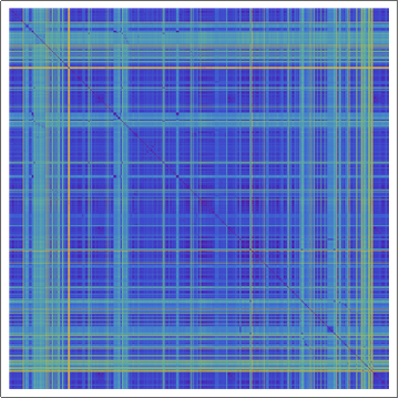
ArrayPlot[dldistance, ColorFunction -> "Rainbow"]
(*Generation of the properties of the Damerau-Levenshtein
distances for the sequences of transmembrane proteins*)
Print[ "Mean Damerau-Levenshtein distance = ",
N[Mean[Flatten[dldistance]]]]
Print["Median Damerau-Levenshtein distance = ",
N[Median[Flatten[dldistance]]]]
Print["SD of the Damerau-Levenshtein distance = ",
N[StandardDeviation[Flatten[dldistance]]]]
Print["Skewness of the Damerau-Levenshtein distance = ",
N[Skewness[Flatten[dldistance]]]]
Mean Damerau-Levenshtein distance = 768.983
Median Damerau-Levenshtein distance = 673.
SD of the Damerau-Levenshtein distance = 423.818
Skewness of the Damerau-Levenshtein distance = 1.47982
In the rainbow color encoded array plot the violet corresponds to the 0 Damerau-Levenshtein distance, as the color changes towards read the Damerau-Levenshtein distance increases. In order to get deeper understanding of the statistical data of protein sequences displayed above we went on and generated random amino acid sequences:
aminoac = {"L", "S", "A", "V", "G", "E", "T", "I", "P", "R", "K", "F",
    "D", "Q", "N", "Y", "C", "M", "H", "W"};

(*Generation of one random amino acid sequence of random length that
is between given integers.*)
generatePolypeptide[m_, n_] :=
 Module[{aminoac = {"L", "S", "A", "V", "G", "E", "T", "I", "P", "R",
     "K", "F", "D", "Q", "N", "Y", "C", "M", "H", "W"}, out},
  out = StringJoin@RandomChoice[aminoac, RandomInteger[{m, n}]]
  ]

(*Generation of several(l) random amino acid sequence of random
length that is between given integers.*)
generatePlist[l_, ps_, pl_] := Module[{out = {}},
  Do[out = AppendTo[out, generatePolypeptide[ps, pl]], l];
  out
  ]

(*Generation of 694 random amino acid sequences that has minimum
length of 55 and maximum length of 3097. Those numbers are the
maximal and minimal lengths of sequences in our transmembrane protein
data.*)
(randomseq = generatePlist[694, 55, 3079]) // Short
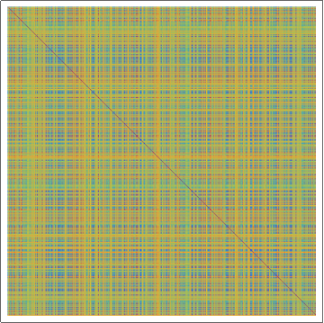
Next we have performed similar operations over this random amino acid sequence data as we did for the transparent protein sequences. Below is rainbow color encoded array plot of the random amino acid sequence data with some statistical characteristics.
(*Computaion of the Damerau\[Dash]Levenshtein distance between the
random amino acid sequences.*)
(*The computaion time is around 120 min*)
dldistanceRand =
  Table[DamerauLevenshteinDistance[randomseq[[j]],
    randomseq[[k]]], {j, 694}, {k, 694}];

(*Showing the Damerau-Levenshtein distance array plot for the
random amino acid sequences, with rainbow colors. Violet means that
sequences are identical.*)
ArrayPlot[dldistanceRand, ColorFunction -> "Rainbow"]
(*Generation of the properties of the Damerau-Levenshtein
distances for the sequences of transmembrane proteins*)
Print[ "Mean Damerau-Levenshtein distance = ",
 N[Mean[Flatten[dldistanceRand]]]]
Print["Median Damerau-Levenshtein distance = ",
 N[Median[Flatten[dldistanceRand]]]]
Print["SD of the Damerau-Levenshtein distance = ",
 N[StandardDeviation[Flatten[dldistanceRand]]]]
Print["Skewness of the Damerau-Levenshtein distance = ",
 N[Skewness[Flatten[dldistanceRand]]]]
Mean Damerau-Levenshtein distance = 1744.85
Median Damerau-Levenshtein distance = 1863.
SD of the Damerau-Levenshtein distance = 578.999
Skewness of the Damerau-Levenshtein distance = -0.613977
From this analysis one can conclude that transmembrane protein sequences are closely related in contrast to random amino acid sequences.
Next we have written a short script that will guess whether the proposed sequence can be a transmembrane protein sequence, try it.
(*Selection of the training data sets*)
{trainTRSeq, testTRSeq} = TakeDrop[trseq, 600];
{trainRandSeq, testRandSeq} = TakeDrop[randomseq, 600];

(*Classification of the transmembrane protein classification*)
(*The computaion time is around 3 min*)
protClassifier =
 Classify[<|"Transmembrane protein sequence" -> trainTRSeq,
   "Not a transmembrane protein sequence" -> testRandSeq|>,
  Method -> "Markov", PerformanceGoal -> "Quality"]

(*Creation of validation set*)
valtrSeq = Thread[testTRSeq -> "Transmembrane protein sequence"];
valRandSeq =
  Thread[testRandSeq -> "Not a transmembrane protein sequence"];
validation = Join[valtrSeq, valRandSeq];

(*Testing the accuracy of the classifier*)
cm = ClassifierMeasurements[protClassifier, validation]
cm["Accuracy"]

(*A decision maker that will tell wehter proposed sequence can be
transmembrane protein seqeunce*)
decision[sequence_] :=
  If [(StringLength[sequence] <
      30) || (Max[
       Abs@ Subtract[#[[1]], #[[2]]] & /@
        StringPosition[sequence, x_ ~~ x_]] > 20),
   "Not a transmembrane protein sequence", protClassifier[sequence]];

FormFunction["Sequence" -> "String", decision[#Sequence] &]
Words in different languages are in some seance similar to protein sequences. Both are products of evolution, but these evolutions have different purposes and driving forces. Using the same codes we have analyzed words in different languages. The word data was obtained as follows (for example for German words):
german = ToLowerCase[
  WordList["KnownWords", Language -> Entity["Language", "German"]]]
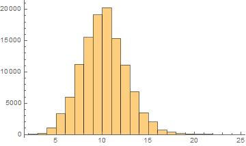
Next are presented word length distributions for few languages:
English
Mean = 8.33284
Median = 8.
SD = 2.64659
Skewness = 0.37119
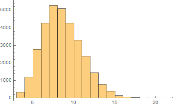
German
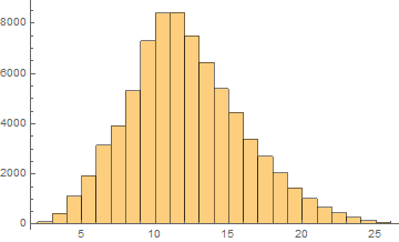
Mean = 11.6281
Median = 11.
SD = 3.95164
Skewness = 0.455154
Italian
Mean = 9.64161
Median = 10.
SD = 2.42446
Skewness = 0.2337
Russian
Mean = 8.10481
Median = 8.
SD = 2.41756
Skewness = 0.44462
Arabic
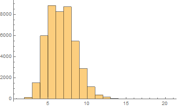
Mean = 6.24913
Median = 6.
SD = 1.83311
Skewness = 0.525033
Hebrew
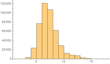
Mean = 6.75852
Median = 7.
SD = 1.77025
Skewness = 0.993837
It can be noticed that the length of words in the Semitic languages that are shown here are relatively shorter. Next we are showing the array plots for DamerauLevenshtein distances calculated between 10000 words for each language.
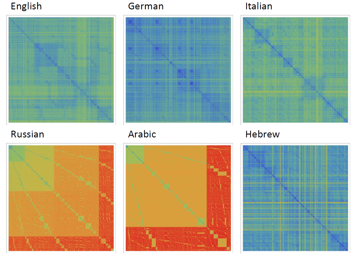
It shows that the DamerauLevenshtein distances between Russian words and Arabic words are large in comparison English, German, Italian and Hebrew. What would be your interpretation of the image above?
 Attachments:


