Group Abstract Group Abstract

Message Boards Message Boards

Best NDSolve Methods for this equation?

Posted 10 years ago
POSTED BY: Fernando Garcia
4 Replies
Posted 10 years ago

This works pretty well. Numeric ....

solpru = NDSolve[{D[y[x, t], t] == -D[D[y[x, t], x], x], 
    y[0, t] == Sin[0], y[Pi, t] == Sin[Pi], y[x, 0] == Sin[x]}, 
   y, {x, 0, Pi}, {t, 0, 1}, MaxSteps -> Infinity, PrecisionGoal -> 3,
    AccuracyGoal -> 8, 
   Method -> {"MethodOfLines", 
     "SpatialDiscretization" -> "FiniteElement"}];

    Plot3D[Evaluate[y[x, t] /. solpru], {x, 0, Pi}, {t, 0, 1}]

enter image description here

Analytical

sol2 = DSolve[{D[y[x, t], t] == -D[y[x, t], {x, 2}], 
y[0, t] == Sin[0], y[Pi, t] == Sin[Pi], y[x, 0] == Sin[x]}, 
y, {x, 0, Pi}, {t, 0, 1}]

{{y -> Function[{x, t}, E^t Sin[x]]}}

analytical

POSTED BY: Eric Meyers

Thank you very much.

The discretization using Finite Elements work for this case. However, I have noticed that the FiniteElement discretization apparently does not work when the coefficients of the equation are not polynomials of the unknowns. For example:

dy/dt = -1/(1+y) d^2 y/dx^2.

Would you know how to overcome this problem?

Thank you!

POSTED BY: Fernando Garcia

Hey. First ,I don't know the best Method options for this type,but this code below works:

ppR = 20;
solpru = NDSolve[{D[y[x, t], t] == -D[D[y[x, t], x], x], 
    y[0, t] == Sin[0], y[Pi, t] == Sin[Pi], y[x, 0] == Sin[x]}, 
   y, {x, 0, Pi}, {t, 0, 1}, MaxSteps -> Infinity, PrecisionGoal -> 1,
    AccuracyGoal -> 1, 
   Method -> {"MethodOfLines", 
     "SpatialDiscretization" -> {"TensorProductGrid", 
       "MinPoints" -> ppR, "MaxPoints" -> ppR, 
       "DifferenceOrder" -> 1}, 
     Method -> {"ExplicitEuler", "MaxDifferenceOrder" -> 4}}];
ys[x_, t_] := Evaluate[y[x, t] /. solpru];
Plot[{ys[x, 0], ys[x, 1/2], ys[x, 3/4], ys[x, 1]}, {x, 0, Pi}, 
 PlotRange -> All]
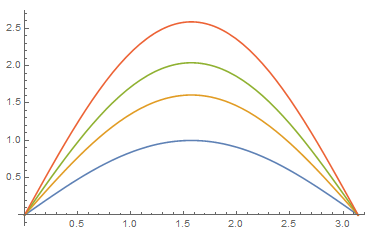
enter image description here

See another code:

ppR = 50;
solpru = NDSolve[{D[y[x, t], t] == -D[D[y[x, t], x], x], 
    y[0, t] == Sin[0], y[Pi, t] == Sin[Pi], y[x, 0] == Sin[x]}, 
   y, {x, 0, Pi}, {t, 0, 1}, MaxSteps -> Infinity, PrecisionGoal -> 1,
    AccuracyGoal -> 1, 
   Method -> {"MethodOfLines", 
     "SpatialDiscretization" -> {"TensorProductGrid", 
       "MinPoints" -> ppR, "MaxPoints" -> ppR, 
       "DifferenceOrder" -> 1}, 
     Method -> {"ImplicitRungeKutta", "DifferenceOrder" -> 2}}];
ys[x_, t_] := Evaluate[y[x, t] /. solpru];
Plot[{ys[x, 0], ys[x, 1/2], ys[x, 3/4], ys[x, 1]}, {x, 0, Pi}, 
 PlotRange -> All]

POSTED BY: Mariusz Iwaniuk

Thank you very much!

I see that the key point here is to lower the requirements on precision and accurary goals.

Comparing with the analytic solution, it turns out that the integration with the Implicit Runge Kutta is better than the Explicit Euler.

Best,

Fernando

POSTED BY: Fernando Garcia
Reply to this discussion
Community posts can be styled and formatted using the Markdown syntax.
Reply Preview
Attachments
Remove
or Discard