Hey.
First ,I don't know the best Method options for this type,but this code below works:
ppR = 20;
solpru = NDSolve[{D[y[x, t], t] == -D[D[y[x, t], x], x],
y[0, t] == Sin[0], y[Pi, t] == Sin[Pi], y[x, 0] == Sin[x]},
y, {x, 0, Pi}, {t, 0, 1}, MaxSteps -> Infinity, PrecisionGoal -> 1,
AccuracyGoal -> 1,
Method -> {"MethodOfLines",
"SpatialDiscretization" -> {"TensorProductGrid",
"MinPoints" -> ppR, "MaxPoints" -> ppR,
"DifferenceOrder" -> 1},
Method -> {"ExplicitEuler", "MaxDifferenceOrder" -> 4}}];
ys[x_, t_] := Evaluate[y[x, t] /. solpru];
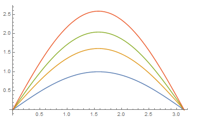
Plot[{ys[x, 0], ys[x, 1/2], ys[x, 3/4], ys[x, 1]}, {x, 0, Pi},
PlotRange -> All]
See another code:
ppR = 50;
solpru = NDSolve[{D[y[x, t], t] == -D[D[y[x, t], x], x],
    y[0, t] == Sin[0], y[Pi, t] == Sin[Pi], y[x, 0] == Sin[x]},
   y, {x, 0, Pi}, {t, 0, 1}, MaxSteps -> Infinity, PrecisionGoal -> 1,
    AccuracyGoal -> 1,
   Method -> {"MethodOfLines",
     "SpatialDiscretization" -> {"TensorProductGrid",
       "MinPoints" -> ppR, "MaxPoints" -> ppR,
       "DifferenceOrder" -> 1},
     Method -> {"ImplicitRungeKutta", "DifferenceOrder" -> 2}}];
ys[x_, t_] := Evaluate[y[x, t] /. solpru];
Plot[{ys[x, 0], ys[x, 1/2], ys[x, 3/4], ys[x, 1]}, {x, 0, Pi},
 PlotRange -> All]


