This is a code I developed last year, while trying to solve an Atari game. The main idea is to go from the initial part of the lattice (A first row) to the last row (B) deviating from obstacles (in this case, cars, black squares). The goal of the model is to find the shortest path between A and B, given the cars in the road. Initially I thought I could use tuples of paths in the 6 x 15 lattice, but the possible options were computationally expensive.

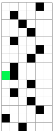
a=Table[Insert[Table[0,{5}],1,RandomInteger[{1,5}]],{15}];

{ArrayPlot[a,Mesh->True,ImageSize->180,Frame->True]}

Green square is car moving:

So I used a Markov Chain Monte Carlo model, using Markov Chains to generate possible paths given spatial restrictions.

b=Partition[Flatten[Position[a[[#]],0]&/@Table[k,{k,1,Dimensions[a][[1]],1}]],5]
h=b[[#]][[RandomInteger[{1,5}]]]&/@Table[k,{k,1,Dimensions[a][[1]],1}]
g1=Flatten[{h[[#]]->h[[#+1]]}&/@Table[k,{k,1,14,1}]]
hh=Insert[a[[#]],2,h[[#]]]&/@Table[k,{k,1,Dimensions[a][[1]],1}]
f1=Delete[hh[[#]],h[[#]]+1]&/@Table[k,{k,1,Dimensions[a][[1]],1}]

{LayeredGraphPlot[g1,VertexLabeling->True,ImageSize->360],Dynamic[j=Clock[{1,15,1},5];{ArrayPlot[bb=Insert[Delete[a,j],f1[[j]],j],Mesh->True,ImageSize->170,ColorRules->{0->White,1->Black,2->Green}],Grid[Insert[Delete[a,j],f1[[j]],j]/.{0->'blank',1->'black car',2->'orange car'}]}]}

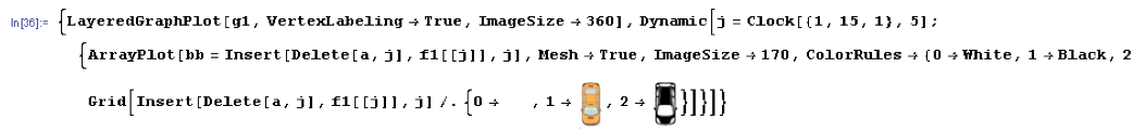
Generating this dynamic output:

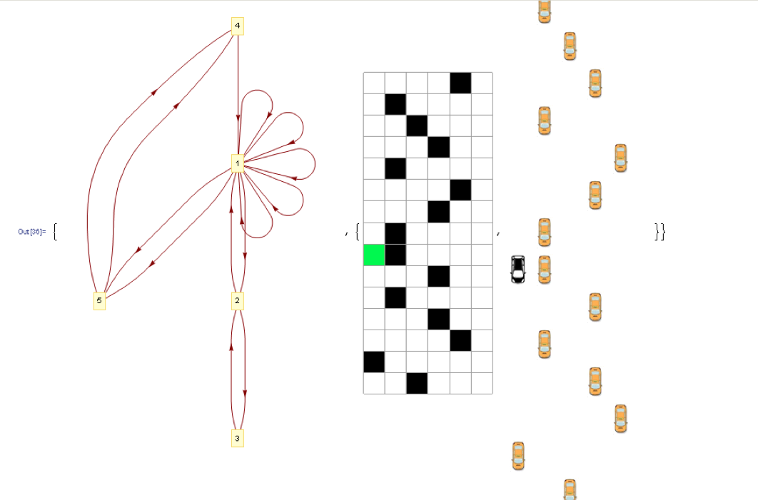
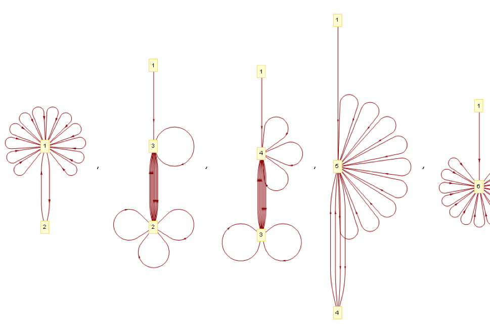
Then the possible paths are shown:

r={b[[1]][[1]],b[[2]][[#]],b[[3]][[#]],b[[4]][[#]],b[[5]][[#]],b[[6]][[#]],b[[7]][[#]],b[[8]][[#]],b[[9]][[#]],b[[10]][[#]],b[[11]][[#]],b[[12]][[#]],b[[13]][[#]],b[[14]][[#]],b[[15]][[#]]}&/@Table[k,{k,1,5,1}]
g12={r[[#]][[1]]->r[[#]][[2]],r[[#]][[2]]->r[[#]][[3]],r[[#]][[3]]->r[[#]][[4]],r[[#]][[4]]->r[[#]][[5]],r[[#]][[5]]->r[[#]][[6]],r[[#]][[6]]->r[[#]][[7]],r[[#]][[7]]->r[[#]][[8]],r[[#]][[8]]->r[[#]][[9]],r[[#]][[9]]->r[[#]][[10]],r[[#]][[10]]->r[[#]][[11]],r[[#]][[11]]->r[[#]][[12]],r[[#]][[12]]->r[[#]][[13]],r[[#]][[13]]->r[[#]][[14]],r[[#]][[14]]->r[[#]][[15]]}&/@Table[k,{k,1,5,1}]
q=LayeredGraphPlot[g12[[#]],VertexLabeling->True,ImageSize->180]&/@Table[k,{k,1,5,1}]

And a Manipulate command is inserted to show car movements in each path:

ft[t_]:=Insert[a[[#]],2,r[[t]][[#]]]&/@Table[k,{k,1,Dimensions[a][[1]],1}]
hh2=ft/@Table[k,{k,1,Dimensions[r][[1]],1}]
gh[ty_]:=Delete[hh2[[ty]][[#]],r[[ty]][[#]]+1]&/@Table[k,{k,1,Dimensions[a][[1]],1}]
f13=gh/@Table[k,{k,1,Dimensions[hh2][[1]],1}]
Manipulate[Dynamic[j=Clock[{1,15,1},5];{ArrayPlot[Insert[Delete[a,j],f13[[ss]][[j]],j],Mesh->True,ImageSize->230,ColorRules->{0->White,1->Black,2->Green}],Grid[Insert[Delete[a,j],f13[[ss]][[j]],j]/.{0->,1->,2->}]}],{ss,1,5,1,Appearance->"Open"}]

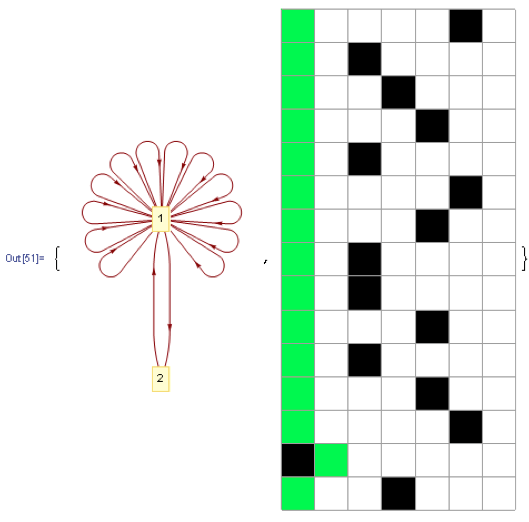
Then the shortest path is chosen:

dg=Total[Abs[{r[[#]][[1]]-r[[#]][[2]],r[[#]][[2]]-r[[#]][[3]],r[[#]][[3]]-r[[#]][[4]],r[[#]][[4]]-r[[#]][[5]]}]]&/@Table[k,{k,1,Dimensions[r][[1]],1}]
Insert[Delete[a,#],f13[[1]][[#]],#]&/@Table[k,{k,1,5,1}]
{q[[Flatten[Position[dg,Min[dg]]][[1]]]],ArrayPlot[hh2[[1]],Mesh->True,ImageSize->220,ColorRules->{0->White,1->Black,2->Green}]}

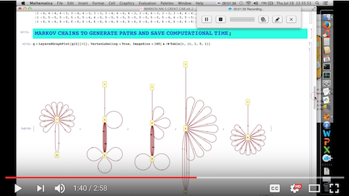
For a video of the output, please access my YouTube video on MCMC: Markov Chain Monte Carlo

Attachments: