Message Boards Message Boards

0
|
9997 Views
|
5 Replies
|
3 Total Likes
View groups...
Share
Share this post:

How to plot the outage probability?

Posted 11 years ago
How to plot the outage probability (f) of the gamma function in empirical distribution (by simulation) and theoretical distribution in the same figure for comparison purpose
f = 1 - Gamma[ m, (m ((2^(2 R) - 1)/S)^(1/n))/ t] (Gamma[m, (m ((2^(2 R) - 1)/S)^(1/n))/t]/Gamma[m]^2)
Plot[f, {S, 0, 7}]

we assume that R=1, n=3, m=1, t=1
POSTED BY: John G
5 Replies
This should work:
f=1-Gamma[m,(m ((2^(2 R)-1)/S)^(1/n))/t] (Gamma[m,(m ((2^(2 R)-1)/S)^(1/n))/t]/Gamma[m]^2)
Plot[f/.{m->1,t->1,n->3,R->1},{S,0,7}]
You have to substiture values for m,t,n,R otherwise you can't plot it.
POSTED BY: Sander Huisman
Posted 11 years ago
Thanks for your interest, but my enquiry is about the comparison between analytical results with simulation results such as the below graph as an example:

 
POSTED BY: John G
What about something like
 f[m_, S_] :=
  With[{ R = 1, n = 3, t = 1},
   1 - Gamma[
      m, (m ((2^(2 R) - 1)/S)^(1/n))/
       t] (Gamma[m, (m ((2^(2 R) - 1)/S)^(1/n))/t]/Gamma[m]^2)]
 
 data = Table[{S, f[#, S] + RandomReal[{-1, 1}]/100}, {S, 0.01,
       7, .1}] & /@ {1, 2, 3};
 
Show[
Plot[Evaluate[f[#, S] & /@ {1, 2, 3}], {S, 0, 7}],
ListPlot[data]
]
In the probability speak, the function f is known as a SurvivalFunction. We can define the probability distribution, describing the outage characteristics (either a duration, or an onset, you are not being specific) as
In[80]:= f = (FullSimplify[#1, S > 0] & )[
FunctionExpand[With[{R = 1, n = 3, m = 1, t = 1},
1 - Gamma[m, (m*((2^(2*R) - 1)/S)^(1/n))/t]*(Gamma[m, (m*((2^(2*R) - 1)/S)^(1/n))/t]/Gamma[m]^2)]]]

Out[80]= 1 - E^(-((2*3^(1/3))/S^(1/3)))

In[81]:= odist =
ProbabilityDistribution[{"SF", f}, {S, 0, Infinity}];

We can now sample from this distribution using RandomVariate:
sample = RandomVariate[dist, 10^6];

The distribution has heavy-tail:
In[52]:= Probability[x > 1000, x \[Distributed] sample] // N

Out[52]= 0.24759

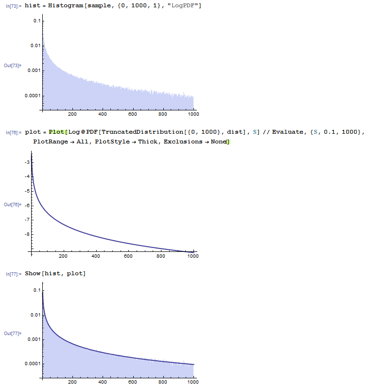
Here we plot a histogram of the data, displaying the logarithm of the probability density function:
hist = Histogram[sample, {0, 1000, 1}, "LogPDF"];
plot = Plot[Log@PDF[TruncatedDistribution[{0, 1000}, dist], S] // Evaluate, {S, 0.1, 1000}, PlotRange -> All, PlotStyle -> Thick, Exclusions -> None];
Show[hist, plot]

Here is a screen-shot:
POSTED BY: Oleksandr Pavlyk
Posted 11 years ago
Hi Oleksandr,

In fact, I am willing to inquire if I can plot the following function with scattered data instead of histogram graph as I want to compare this with the analytical graph below
f = Product[ 1 - (Gamma[m, (m ((2.25)/10^(S/10))^(1/n))/\[CapitalOmega]] Gamma[ m, (m ((1.5)/10^(S/10) )^(1/n))/\[CapitalOmega]])/ Gamma[m]^2, {i, 1, M}] /. Subscript -> Part;
ticks = {10^-4, 10^-3, 10^-2, 10^-1, 1};
LogPlot[f, {S, 0, 40}, PlotRange -> {10^-4, 1}, Ticks -> {Automatic, ticks}, GridLines -> Automatic, Frame -> True]
Assuming that :
m=1, n=1, M=3, \[CapitalOmega] = 2
POSTED BY: John G
Reply to this discussion
Community posts can be styled and formatted using the Markdown syntax.
Reply Preview
Attachments
Remove
or Discard

Group Abstract Group Abstract