Decomposition Approach
ABSTRACT
Seasonality in economic data plays important part in econometric forecasting and predictions for future business decisions. In this respect, understanding and estimation of seasonality patterns in inflation data is essential component of pricing decisions for any payoffs linked to inflation. We present decomposition method for inflation seasonality detection a simple, but robust technique for seasonality detection. Thanks for to flexibility of powerful Wolfram Programming Language, the implementation is quick and efficient with accomplishment in just few steps
Seasonality in economic data
Economic time series are known to exhibit fluctuation and distortions. These tend to occur in periodic intervals. Fluctuations that last several years and occur in regular intervals are know as business cycles, whereas variations driven by seasonal characteristics and occurring typically within a year are called seasonality. The understanding of seasonality is important because many business and economic data are seasonal. Seasonality, especially when strong, can hide important features such as trends and cyclicity, and therefore proper understanding of seasonality is important pre-requisite for understanding time series. If seasonality is material, its detection and anticipation can male different between correct and incorrect business decision.
Seasonality is typical feature of GDP measurement, labor statistics, retail sales, construction activity and strongly characterizes inflation processes. This is the primary focus of this analysis.
Seasonality can be measured in several ways. We examine first the so-called decomposition methods, which are one of the oldest techniques in econometric modeling and forecasting.
Time series components
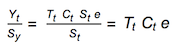
Time series can be decomposed into a set of fundamental components with its own unique characteristic. In the basic format, the time series at any point of time Subscript[Y, t] can be expressed as multi-factors model:
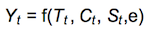
where f denotes the model's function, T is the trend, C is the cyclical component, S is the seasonality influence and e is the error term.
Trend and cyclical factors represent a 'growth' pattern in time series, and usually are modelled together. MutiThis is because a separation of trend from cyclicality is not simple. Although seasonality can be formulated on any time interval, quarterly and monthly variations are most common. The error term is a residual component of time series that is not explained by trend, cycle or seasonality. It's random and thus unpredictable.
Decomposition models
There are tow major decomposition models:
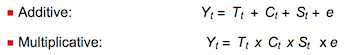
DecoThe choice of the model depends on the nature of time series. If the plot of the data revelers the independence of seasonality and cycle from the general level, then using additive model is a right decision. However, when factors are dependent on each other (eg. seasonality varies due to the trend / cycle), choosing multiplicative model is a right strategy to follow.
Multiplicative model is more common in the econometric studies and is also a preferred choice for extraction of inflation seasonality.
Multiplicative seasonal model
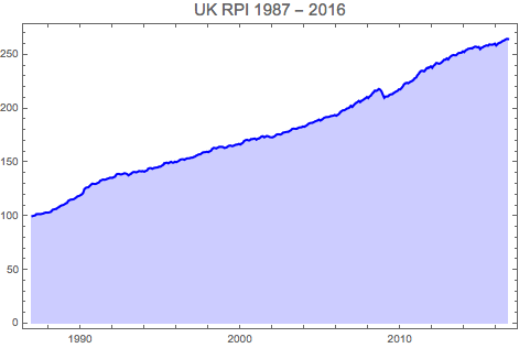
Decomposition method for multiplicative model uses the ratio of moving averages and centered smoothing to determine seasonal factors. We will demonstrate the approach on the UK RPI data.
We take the UK RPI history from Jan 1987 up to Oct 2016 and create the time series object
ukrpi = {100, 100.4, 100.6, 101.8, 101.9, 101.9, 101.8, 102.1, 102.4,
   102.9, 103.4, 103.3, 103.3, 103.7, 104.1, 105.8, 106.2, 106.6,
   106.7, 107.9, 108.4, 109.5, 110, 110.3, 111, 111.8, 112.3, 114.3,
   115, 115.4, 115.5, 115.8, 116.6, 117.5, 118.5, 118.8, 119.5, 120.2,
    121.4, 125.1, 126.2, 126.7, 126.8, 128.1, 129.3, 130.3, 130,
   129.9, 130.2, 130.9, 131.4, 133.1, 133.5, 134.1, 133.8, 134.1,
   134.6, 135.1, 135.6, 135.7, 135.6, 136.3, 136.7, 138.8, 139.3,
   139.3, 138.8, 138.9, 139.4, 139.9, 139.7, 139.2, 137.9, 138.8,
   139.3, 140.6, 141.1, 141, 140.7, 141.3, 141.9, 141.8, 141.6, 141.9,
    141.3, 142.1, 142.5, 144.2, 144.7, 144.7, 144, 144.7, 145, 145.2,
   145.3, 146, 146, 146.9, 147.5, 149, 149.6, 149.8, 149.1, 149.9,
   150.6, 149.8, 149.8, 150.7, 150.2, 150.9, 151.5, 152.6, 152.9, 153,
    152.4, 153.1, 153.8, 153.8, 153.9, 154.4, 154.4, 155, 155.4,
   156.3, 156.9, 157.5, 157.5, 158.5, 159.3, 159.5, 159.6, 160, 159.5,
    160.3, 160.8, 162.6, 163.5, 163.4, 163, 163.7, 164.4, 164.5,
   164.4, 164.4, 163.4, 163.7, 164.1, 165.2, 165.6, 165.6, 165.1,
   165.5, 166.2, 166.5, 166.7, 167.3, 166.6, 167.5, 168.4, 170.1,
   170.7, 171.1, 170.5, 170.5, 171.7, 171.6, 172.1, 172.2, 171.1, 172,
    172.2, 173.1, 174.2, 174.4, 173.3, 174, 174.6, 174.3, 173.6,
   173.4, 173.3, 173.8, 174.5, 175.7, 176.2, 176.2, 175.9, 176.4,
   177.6, 177.9, 178.2, 178.5, 178.4, 179.3, 179.9, 181.2, 181.5,
   181.3, 181.3, 181.6, 182.5, 182.6, 182.7, 183.5, 183.1, 183.8,
   184.6, 185.7, 186.5, 186.8, 186.8, 187.4, 188.1, 188.6, 189, 189.9,
    188.9, 189.6, 190.5, 191.6, 192, 192.2, 192.2, 192.6, 193.1,
   193.3, 193.6, 194.1, 193.4, 194.2, 195, 196.5, 197.7, 198.5, 198.5,
    199.2, 200.1, 200.4, 201.1, 202.7, 201.6, 203.1, 204.4, 205.4,
   206.2, 207.3, 206.1, 207.3, 208, 208.9, 209.7, 210.9, 209.8, 211.4,
    212.1, 214, 215.1, 216.8, 216.5, 217.2, 218.4, 217.7, 216, 212.9,
   210.1, 211.4, 211.3, 211.5, 212.8, 213.4, 213.4, 214.4, 215.3, 216,
    216.6, 218, 217.9, 219.2, 220.7, 222.8, 223.6, 224.1, 223.6,
   224.5, 225.3, 225.8, 226.8, 228.4, 229, 231.3, 232.5, 234.4, 235.2,
    235.2, 234.7, 236.1, 237.9, 238, 238.5, 239.4, 238, 239.9, 240.8,
   242.5, 242.4, 241.8, 242.1, 243, 244.2, 245.6, 245.6, 246.8, 245.8,
    247.6, 248.7, 249.5, 250, 249.7, 249.7, 251, 251.9, 251.9, 252.1,
   253.4, 252.6, 254.2, 254.8, 255.7, 255.9, 256.3, 256, 257, 257.6,
   257.7, 257.1, 257.5, 255.4, 256.7, 257.1, 258, 258.5, 258.9, 258.6,
    259.8, 259.6, 259.5, 259.8, 260.6, 258.8, 260, 261.1, 261.4,
   262.1, 263.1, 263.4, 264.4, 264.9, 264.8};
rpits = TimeSeries[ukrpi, {{1987, 1, 1}, {2016, 10, 1}, "Month"}];
DateListPlot[rpits, PlotLabel -> Style["UK RPI 1987 - 2016", 15],
 PlotStyle -> {Blue, Thick}, Filling -> Axis]
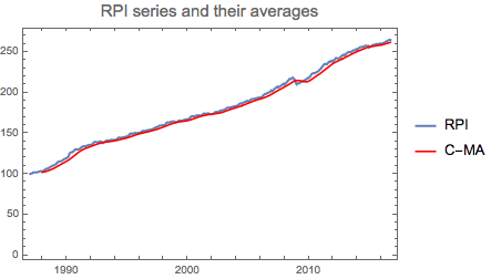
To proceed with seasonality calculation, we apply the moving average (MA) technique twice:
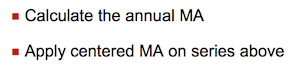
mova1 = MovingAverage[rpits, 12];
mova2 = MovingAverage[mova1, 2];
DateListPlot[{rpits, mova2},
 PlotLabel -> Style["RPI series and their averages", 15],
 PlotLegends -> {"RPI", "C-MA"}, PlotStyle -> {Thick, {Blue, Red}}]
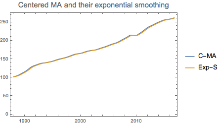
The use of centered moving averages is practical, but not exhaustive and we can apply further smoothing techniques to adjust the data. Exponential smoothing is one of them.
mova3 = ExponentialMovingAverage[mova2, 0.25];
DateListPlot[{mova2, mova3},
 PlotLabel -> Style["Centered MA and their exponential smoothing", 15],
 PlotLegends -> {"C-MA", "Exp-S"}]
In the next steps we calculate the ratio of moving averages where the original series are divided by their MA
newrpi=TimeSeriesWindow[rpits,{mova3["FirstTime"],{2016,10,1}}];
rat1=newrpi/mova3;
DateListPlot[rat1,PlotLabel->Style["Ratio of MA",15],Filling->Axis]
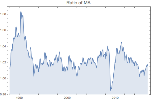
The ratio above is essentially the S*e quantity obtained from time series. To eliminate the randomness from the data, we simply average the value over the 12-monthly intervals.
rawseas=Table[Mean[Take[rat1["Values"],{i,Length[rat1["Values"]],12}]],{i,1,12}]
{1.0179878778325224,1.020865454219894,1.0220704288011477,1.0283140969748503, 1.0292781053076343,1.0282757052368627,1.0237944649874124,1.0252818857730472, 1.0269539388642832,1.025905611864363,1.0244253764240674,1.024069255746688}
The 'raw' seasonal indices are the first-level results we aim to achieve. We perform further adjustment to the indices to ensure they sum up to 12
rpiseas=(12/Total[rawseas])*rawseas
lab={"Jan","Feb","Mar","Apr","May","Jun","Jul","Aug","Sep","Oct","Nov","Dec"};
DateListPlot[rpiseas,{2015,1},PlotLabel->Style["UK PRI Seasonal Indices",15],
PlotStyle->{Red,Thick},Mesh->Full,PlotMarkers->Automatic, InterpolationOrder->1,ImageSize->400]
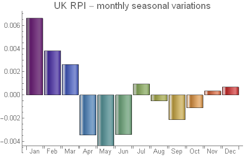
BarChart[{1-rpiseas},ChartElementFunction->"GlassRectangle",ChartStyle->"Rainbow",
ChartLabels->lab,PlotLabel->Style["UK RPI - monthly seasonal variations",15],ImageSize->400]
{0.993383, 0.996191, 0.997367, 1.00346, 1.0044, 1.00342, 0.999049, 1.0005, 1.00213, 1.00111, 0.999665, 0.999318}
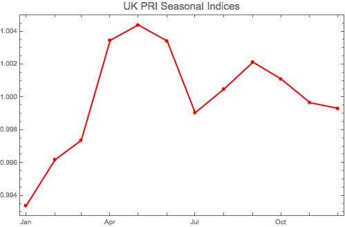
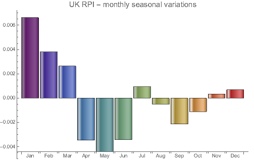
What does the result tell us? The UK RPI seasonality tends to be low in the first quarter of the year, then higher in the second quarter and mixed in the second half of the year.
De-seasonalising inflation data
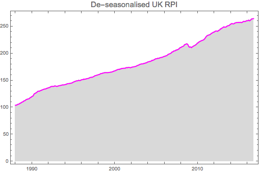
Having obtained the seasonal indices, we can now de-seasonalise the RPI data. From the decomposition formula this is simply
deseasRpi = newrpi["Values"]/PadRight[rpiseas,Length[newrpi["Values"]],rpiseas];
DateListPlot[deseasRpi,{1988,1},PlotLabel->Style["De-seasonalised UK RPI",15],
PlotStyle->{Magenta,Thick},Filling->Axis,FillingStyle->LightGray]
Obtaining the trend for inflation data
Once the de-seasonalised series are available, we can proceed further and estimate the trend and cyclicality in the inflation data.
Trends can be usually estimated with some regression techniques, with Linear being the simplest. Mathematica, however, offers more elegant solutions. Two alternatives include:
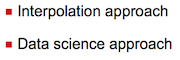
Interpolation
We can choose from few alternatives in terms of order. Linear or Quadratic model will fit the RPI data well.
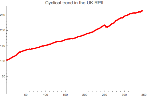
trendInt = ListInterpolation[deseasRpi, InterpolationOrder -> 2,
  Method -> "Spline"]; ListLinePlot[trendInt,
 PlotLabel -> Style["Cyclical trend in the UK RPII", 15],
 PlotStyle -> {Red, Thickness[0.009]}]
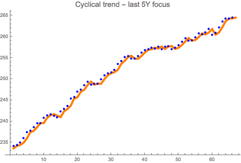
ListPlot[{Take[deseasRpi, -66], Table[trendInt[i], {i, 280, 346}]},
 PlotStyle -> {Blue, {Orange, Thickness[0.009]}}, Joined -> {False, True},
 PlotLabel -> Style["Cyclical trend - last 5Y focus", 15]]
Data science route
We can also use the most recent advances in Mathematica and use the new function FindFormula that tries to find symbolic function to the underlying data.
trendFrm = FindFormula[deseasRpi, t]
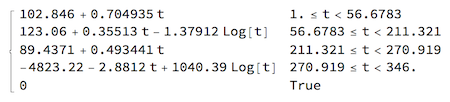
Automatic fit finds the piecewise formula that can be easily applied to visualize and generate functional data.
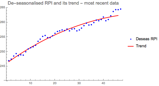
ListPlot[{Take[deseasRpi, -47], Table[trendFrm, {t, 300, 345}]},
 Joined -> {False, True}, PlotLabel -> Style["De-seasonalised RPI and its trend - most recent data", 15],
 PlotStyle -> {Blue, {Red, Thick}}, PlotRange -> {240, 265},
 PlotLegends -> {"Deseas RPI", "Trend"}, ImageSize -> 400]
Additive seasonal model
Methods and steps devised in the multiplicative seasonal model can be re-applied in the additive model that instead of division and multiplication operates on subtraction and addition. We will perform the following steps:
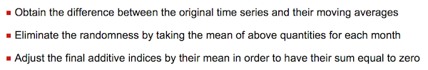
addDiff=newrpi-mova3;
rawseasadd=Table[Mean[Take[addDiff["Values"],{i,Length[addDiff["Values"]],12}]],{i,1,12}];
rpiseasadd=rawseasadd-Mean[rawseasadd]
{-1.22689, -0.661592, -0.42587, 0.535942, 0.713983, 0.569999, -0.172041, 0.122327, 0.432471, 0.234763, -0.0640571, -0.0590322}
We can verify the correctness of the calculation by ensuring:
a) sum of additive seasonalities is equal to zero
b) average of all additive seasonalities is zero as well
{Total[rpiseasadd], Mean[rpiseasadd]} // Round
{0, 0}
DateListPlot[rpiseasadd,{1015,1},PlotStyle->{Magenta,Thick},Mesh->Full,PlotMarkers->Automatic,
    InterpolationOrder->1, PlotLabel->Style["Additive UK RPI seasonalities",15],ImageSize->400]
BarChart[{rpiseasadd},ChartElementFunction->"GlassRectangle",ChartStyle->"TemperatureMap",
    ChartLabels->lab,PlotLabel->Style["UK RPI variations", 15],ImageSize->400]
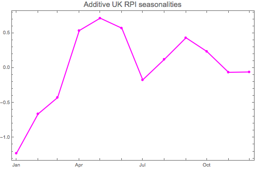
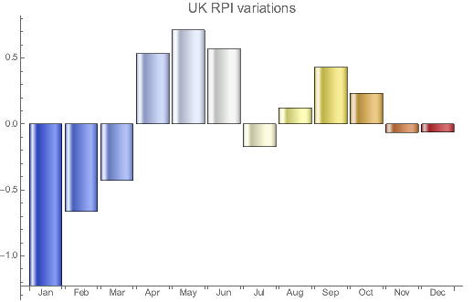
It is not surprising to see the additive seasonalities being similar to the multiplicative ones. This shows both models identify similar seasonality characteristics that govern UK RPI series over the longer interval.
Regression approach in decomposition methods
Regression technique is a flexible technique for finding relationship between data, and, as such, can also be used to model seasonality in inflation series. When seasonality is modelled through regression, all series components have to be defined as as regression variables that influence the response. In this respect, we define (i) trend and (ii) 11 monthly seasonal variables that we egress against the RPI series.
For the regression model, we choose shorter series pattern with 16 years of PRI data
rpireg = TimeSeriesWindow[rpits, {{2000, 1, 1}, {2015, 12, 1}}];
vals = rpireg["Values"];
We create table of data in the matrix format 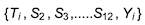
tbl1 = Table[If[i == j, 1, 0], {i, 0, 11}, {j, 1, 11}];
tbl2 = Table[tbl1, {16}];
tbl3 = Flatten[tbl2, 1];
tbl4 = MapThread[Prepend, {tbl3, Range[16*12]}];
tbl5 = MapThread[Append, {tbl4, vals}];
tbl6 = MapThread[Append, {tbl4, Log[vals]}];
vars = {T, S2, S3, S4, S5, S6, S7, S8, S9, S10, S11, S12};
We now apply the multi-variate regression for the data
Regression model for additive seasonality
lmod2add = LinearModelFit[tbl5, vars, vars]

lmod2add // Normal
159.04 + 1.16312 S10 + 0.802768 S11 + 0.879919 S12 + 0.720902 S2 +
0.973054 S3 + 1.70646 S4 + 1.85236 S5 + 1.66701 S6 + 0.837911 S7 +
1.10881 S8 + 1.44846 S9 + 0.529098 T
We can now visualize the seasonality data
lmod2add["ParameterTableEntries"];
Take[%,All,1]//Flatten;
aregseas=Drop[%,1];
aregseas-Mean[aregseas];
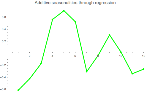
ListLinePlot[%,PlotStyle->{Green,Thickness[0.006]},Mesh->Full,
PlotLabel->Style["Additive seasonalities through regression",15],
PlotMarkers->Automatic, InterpolationOrder->1,ImageSize->400]
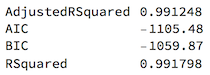
We can look at goodness-of-fit statistics to check the quality of the model
Grid[Transpose[{#, lmod2add[#]} &[{"AdjustedRSquared", "AIC", "BIC", "RSquared"}]], Alignment -> Left]
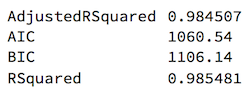
The additive model fits the data quite well which is confirmed by high level of R-Squared statistics.
Regression model for multiplicative seasonality
Multiplicative model uses the same set of market data, with only change being the response vector that is transformed though a Log function
lmod2mul = LinearModelFit[tbl6, vars, vars]

lmod2mul // Normal
5.09571 + 0.00568329 S10 + 0.00399881 S11 + 0.00423331 S12 + 0.00336445 S2 + 0.00463021 S3 + 0.00826615 S4 + 0.00908784 S5 + 0.0082519 S6 + 0.00423283 S7 + 0.00537755 S8 + 0.00707623 S9 + 0.00250739 T
lmod2mul["ParameterTableEntries"];
Take[%, All, 1] // Flatten;
mregseas = Exp[Drop[%, 1]];
mregseas = (12/Total[mregseas])*mregseas;
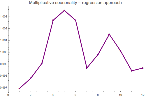
ListLinePlot[mregseas, PlotStyle -> {Purple, Thickness[0.006]},
Mesh -> Full, PlotMarkers -> Automatic, InterpolationOrder -> 1, ImageSize -> 400,
PlotLabel -> Style["Multiplicative seasonality - regression approach", 15]]
We check the goodness-of-fit for the model:
Grid[Transpose[{#, lmod2mul[#]} &[{"AdjustedRSquared", "AIC", "BIC", "RSquared"}]], Alignment -> Left]
We observe even better fit for the multiplicative regression model with high R^2. This confirms that inflation seasonality is better modeled with multiplicative model than the additive one.
Conclusion
Decomposition method for time series is easy-to-apply technique that is well suited for inflation analysis with clear-cut seasonality output. Factorisation of inflation data into components allows quick identification of series drivers and detection of seasonality patterns which in turn affects forecasting. Although the decomposition is simple relative to more advanced seasonality models, it still provides desirable results that we well understory amongst market practitioners.
Decomposition, as this demonstration shows, is easily implemented in Mathematica where only few steps are required to generate seasonality indices from historical series.
 Attachments:


