Hi
I want to merge two adjacent regions in a labelled image witch it obtained by applying watershid algorithm. What should be the best way to do it ?
thanks
Hi Salma,
one way to merge those regions might be to give them identical indices. This could be done by a simple replacement. Here comes an example:
nn = 7;
data = RandomReal[1, {nn, nn}];
f = ListInterpolation[data];
(* test image: *)
img = DensityPlot[f[x, y], {x, 1, nn}, {y, 1, nn}, ImagePadding -> None,
  Frame -> None, ColorFunction -> GrayLevel]
(* water shed components of image *)
wsc0 = WatershedComponents[img];
(* example: merging regions with indices {8,9,10,11} *)
wsc1 = wsc0 /. {8 -> 11, 9 -> 11, 10 -> 11};
You can convince yourself that the result is meaningful:
Plot3D[f[x, y], {x, 1, nn}, {y, 1, nn}, ImageSize -> 700,
 PlotStyle -> Directive[Specularity[White, 100], Texture[Colorize@wsc1]],
 PlotPoints -> 50, MeshFunctions -> {#3 &}]
which gives (e.g.):

Regards – Henrik
I am afraid my answer above is incomplete: There are still the 0s in the index matrix within the merged regions - as can be seen as black lines in the plot. I tried to solve this problem, but my code is lengthy and by no means elegant:
ClearAll["Global`*"]
nn = 7;
data = RandomReal[1, {nn, nn}];
f = ListInterpolation[data];
(*test image:*)
img = DensityPlot[f[x, y], {x, 1, nn}, {y, 1, nn}, ImagePadding -> None,
  Frame -> None, ColorFunction -> GrayLevel]
(*water shed components of image*)
wsc0 = WatershedComponents[img];
(*example: merging regions with indices {8,9,10, (indx=)11}*)
indx = 11;
wsc1 = wsc0 /. {8 -> indx, 9 -> indx, 10 -> indx};

(* ensure there are no 0s at border pixel: *)
wsc1Pad = ArrayPad[wsc1, 1, -1];
(* detect 0-pixels: *)
nullIdx = First /@ Select[Flatten[MapIndexed[{#2, #1} &, wsc1Pad, {2}], 1], Last[#] == 0 &];

(* helper function for counting indx-pixels around coord *)
nearIndxCount[coord_, indx_] := Module[{nears},
  nears = coord + # & /@ {{-1, -1}, {0, -1}, {1, -1}, {-1, 0}, {1, 0}, {-1, 1}, {0, 1}, {1, 1}};
  Count[Extract[wsc1Pad, nears], indx]
  ]

betweens = First /@ Select[{#, nearIndxCount[#, indx]} & /@ nullIdx, Last[#] > 3 &];
Set[wsc1Pad[[Sequence @@ #]], indx] & /@ betweens;
(* remove padding: *)
wsc1 = ArrayPad[wsc1Pad, -1];

Plot3D[f[x, y], {x, 1, nn}, {y, 1, nn}, ImageSize -> 700,
 PlotStyle -> Directive[Specularity[White, 100], Texture[Colorize@wsc1]], PlotPoints -> 50, MeshFunctions -> {#3 &}]
Most likely someone else has a better idea, regards – Henrik
It gradually becomes embarrassing: As I just dicovered, when
wsc0 = WatershedComponents[img, Method -> "Basins"];
is used, there are no 0s i.e. black lines at all!
Dear Henrik,
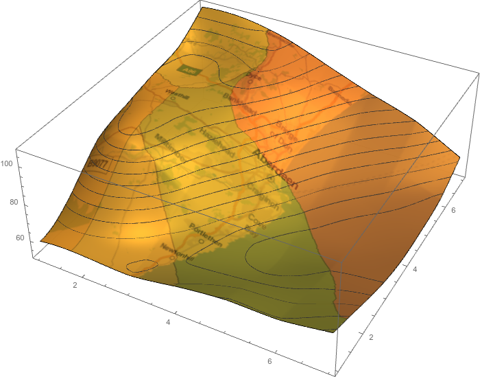
very nice indeed! What a beautiful contribution. I had a group of students this year who modelled rainfall-runoff from some digital elevation data. Your “mountain landscape” looks really nice for that. Here is the result for Aberdeen (UK)
ClearAll["Global`*"]
nn = 7;
data = QuantityMagnitude[
   GeoElevationData[
    GeoDisk[Entity[
      "City", {"Aberdeen", "AberdeenCity", "UnitedKingdom"}],
     Quantity[10, "Miles"]]]];
f = ListInterpolation[data];
(*test image:*)
img =
 DensityPlot[f[x, y], {x, 1, nn}, {y, 1, nn}, ImagePadding -> None,
  Frame -> None, ColorFunction -> GrayLevel]

(*water shed components of image*)
wsc0 = WatershedComponents[img];
(*example:merging regions with indices {8,9,10,(indx=)11}*)

indx = 11;
wsc1 = wsc0 /. {8 -> indx, 9 -> indx, 10 -> indx};

(*ensure there are no 0s at border pixel:*)

wsc1Pad = ArrayPad[wsc1, 1, -1];
(*detect 0-pixels:*)

nullIdx =
  First /@ Select[Flatten[MapIndexed[{#2, #1} &, wsc1Pad, {2}], 1],
    Last[#] == 0 &];

(*helper function for counting indx-pixels around coord*)

nearIndxCount[coord_, indx_] :=
 Module[{nears},
  nears = coord + # & /@ {{-1, -1}, {0, -1}, {1, -1}, {-1, 0}, {1,
      0}, {-1, 1}, {0, 1}, {1, 1}};
  Count[Extract[wsc1Pad, nears], indx]]

betweens =
  First /@ Select[{#, nearIndxCount[#, indx]} & /@ nullIdx,
    Last[#] > 3 &];
Set[wsc1Pad[[Sequence @@ #]], indx] & /@ betweens;
(*remove padding:*)
wsc1 = ArrayPad[wsc1Pad, -1];

Plot3D[f[x, y], {x, 1, nn}, {y, 1, nn}, ImageSize -> 700,
 PlotStyle ->
  Directive[Specularity[White, 100], Texture[Colorize@wsc1]],
 PlotPoints -> 50, MeshFunctions -> {#3 &}]

Plot3D[f[x, y], {x, 1, nn}, {y, 1, nn}, ImageSize -> 700,
 PlotStyle ->
  Directive[Specularity[White, 100],
   Texture[ImageCompose[{Colorize@wsc1,
      0.95}, {GeoGraphics[{GeoStyling[Opacity[0.0]],
        GeoDisk[Entity[
          "City", {"Aberdeen", "AberdeenCity", "UnitedKingdom"}],
         Quantity[10, "Miles"]]}, GeoBackground -> "ReliefMap"],
      0.65}]]], PlotPoints -> 100, MeshFunctions -> {#3 &}]

Thanks for posting!
Cheers,
M.
PS: I kept the black lines, because I like them.
Dear Marco,
nice idea to use GeoElevationData as a 2D scanario, thanks for posting as well! On my system (MM 10.3.1, Linux) the option GeoBackground -> "ReliefMap" is not working - it freezes my MM notebook completely. But the output without that option is also not bad: Aberdeen seems to be located on a hillside towards the sea - very nice!

But then it becomes obvious that the elevation data do not agree very well with the geographical situation …
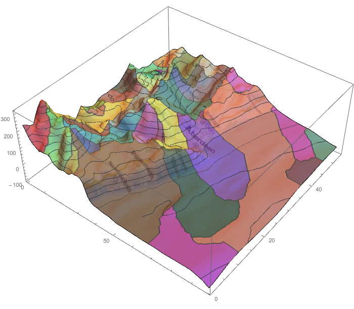
It took me a while to discover the problem: It was the discretization of DensityPlot. For sake of completeness here a combination of our code:
ClearAll["Global`*"]

data = QuantityMagnitude[
   GeoElevationData[
    GeoDisk[Entity[
      "City", {"Aberdeen", "AberdeenCity", "UnitedKingdom"}],
     Quantity[10, "Miles"]]]];
f = ListInterpolation[Reverse@data, InterpolationOrder -> 0];
(*test image:*)
img =
 DensityPlot[f[x, y], {y, 1, 97}, {x, 1, 53}, ImagePadding -> None,
  Frame -> None, ColorFunction -> GrayLevel]
wsc0 = WatershedComponents[img];
texture =
 ImageCompose[{Colorize@wsc0,
   0.95}, {GeoGraphics[{GeoStyling[Opacity[0.0]],
     GeoDisk[Entity[
       "City", {"Aberdeen", "AberdeenCity", "UnitedKingdom"}],
      Quantity[10, "Miles"]]}], 0.35}]
ListPlot3D[Reverse@data, PlotStyle -> Directive[Texture[texture]],
 MeshFunctions -> {#3 &}, ImageSize -> 700]
which now gives:

Best regards from rainy Bavaria – Henrik
[1]: http://community.wolfram.com//c/portal/getImageAttachment?filename=aberdeen.png&userId=32203
[2]: http://community.wolfram.com//c/portal/getImageAttachment?filename=aberdeen1.png&userId=32203
Dear Henrik,
you are absolutely right. I chose a very poor resolution and the plot you generate looks much better and more believable. It is actually very nice for textbooks…
Here is one little thought. Very often mountainous landscapes are described by fractals. The basic idea is that you start, say with a triangle and choose a new point say in the middle of the triangle and move it slightly upward or downwards. Then you iterate. The result looks a bit like this. We first define a function iterate to generate three triangles from one.
iterate[tri_, k_] :=
 Module[{}, noise = {0.2 ( RandomReal[] - 0.1)/k^1.5, 0.2 (RandomReal[] - 0.1)/k^1., 0.5 (RandomReal[] - 0.25)/k^1.5};
  Append[#, RegionCentroid[Triangle[tri]] + noise] & /@ Subsets[tri, {2}]]
Then we iterate, here 8 times:
triangles = {{{0, 0, 0}, {1, 0, 0}, {1/2, Sqrt[2]/2, 0}}}; Do[triangles = Flatten[#, 1] & @(iterate[#, k] & /@ triangles);, {k, 1, 8}]
We can plot this as little triangles, but it doesn’t look very nice:
Graphics3D[{Brown, Triangle[#], EdgeForm[]} & /@ triangles, AspectRatio -> 1, Boxed -> False]

It does look much better when plotted using ListPlot3D:
ListPlot3D[Flatten[triangles, 1], Mesh -> None, ColorFunction -> ColorData["SandyTerrain"], Boxed -> False, Axes -> False, ImageSize -> Full, MaxPlotPoints -> 200]

The exact shape depends a lot on the parameters I choose in the function “iterate”. Perhaps @Vitaliy Kaurov has an idea of how to make this a bit nicer?
Anyway, if you run your algorithm on different “resolutions”, i.e. after iterating a different number of times, the results will look very different. This fractal model, as unrealistic as it is, provides a potential approach to see how many “basins of attraction” or catchment areas you get when you use better resolutions of the terrain data.
I don’t think that I am making myself clear - sorry for that.
Here in Aberdeen there was some snow this morning (23 April, anniversary of Shakespeare’s death).
All the best from the north of (what is still) Europe,
Marco
As you found out, WatershedComponents typically over-segments, yielding too many “regions” as you call them, or components to follow our terminology.
To overcome the issue, you can pre-process the image, or use markers — the documentation shows that extensively. That way the result won’t need merging.
You can also use the “MinimumSaliency” method (see the Options>Method example in WatershedComponents: Image watershed segmentation—Wolfram Documentation). This method essentially produces an over-segmented result first, and then merges neighboring components based on their properties (e.g., areas, distributions of pixel intensities, height of the “pass” between the components, …).
If you’d like to do it yourself, you could start y computing properties for each component:
prop = ComponentMeasurements[{comp, g}, {"Count", "Mean", "Neighbors"}];
and then keep merging the most mergeable component (say, the smallest) with its neighbor that is the nearest to it based on criteria you define (say, the mean intensity should be close enough).