Introduction

I take my coffee black, so I had no idea that there was a large controversy behind when you should add your milk to your coffee. @Gary Bass however highlighted us to this with his question in the community. Apparently, the timing of the added milk is critical. If you add the milk directly the coffee will retain its temperature for a longer time, which is perfect if you plan on drinking later. If you are short on time however, and want to save your throat from scalding hot coffee, you might want to save the milk for just before you are about to drink it.

Obviously, this is something that cannot be taken lightly and some serious simulation is required. I compiled the information from that thread here, for anyone looking to perfect their morning routine. The post will include an explanation for how the model was created. I also however attached the actual model so if you are just looking for the simulation, check out the summary. Hopefully however, you also gain some insights into how to model events involving states in SystemModeler:

Adding Milk to Coffee

In SystemModeler, there are at least two approaches you could take when adding the milk to the coffee. Either you could have everything collected into a single component that has a event in it corresponding to the addition of the milk, or you could have a separate component that specifies the addition of milk as a flow over time. I explored both those scenarios in the attached model.

Approach 1, with a discrete event in the coffee involves creating a copy of the HeatCapacitor component and adding some parameters that separates the heat capacity of the milk, the amount of milk added, when it is added, etc. As you say, the mixed Cp is unknown. A naïve initial approach could be to just add the two heat capacities together. If C is the total heat capacity of the coffee, with or without milk, you could add an equation that says:

  C = if time > AddTime then Ccoffee * Vcoffee * 1000 + Cmilk * Vmilk * 1000 else Ccoffee * Vcoffee * 1000;

The coefficients are just there to convert the different units.

The temperature is a bit more difficult, since it varies continuously over time it is state so and can't be as easily changed as the capacity (which changes values only at one discrete interval).

What you have to do with states is using the reinit(var,newValue) function to reinitialize variable var, to the new value newValue. If you mix fluids together, the new temperature is the new total enthalpy divided by the new heat capacity:

t = (m1 c1 t1 + m2 c2 t2 + ... + mn cn tn) / (m1 c1 + m2 c2 + ... + mn cn)

(from Engineering Toolbox)

In Modelica, we could reinitialize the temperature when the simulation time exceeds the time when the milk should be added, using the following:

  when time > AddTime then
    reinit(T, (Ccoffee * Vcoffee * 1000 * T + Cmilk * Vmilk * 1000 * MilkTemperature) / C);
  end when;

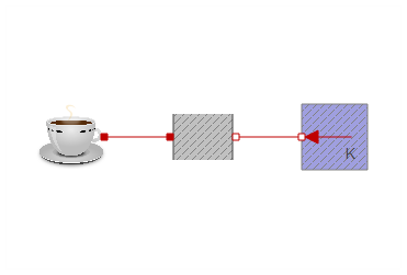
Adding the coffee component and connecting it to a ThermalConductor component (to represent the cup) and connecting that in turn to an FixedTemperature component (to represent the room temperature) results in a fairly compact model:

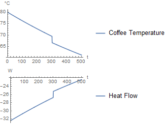
If milk is added after 300 seconds, it produces the following simulation:

Approach 2 is having a short flow of milk, instead of a instantaneous addition of milk. The benefit of this is you could create your own addition strategy. For example, you could add half of the milk at the beginning, and half after 300 seconds. Or any arbitrary strategy. For now, I focused on doing it as a 1 second pulse.

An input is added to the coffee, corresponding to the flow of milk. The volume of the milk in the coffee is no longer a parameter but increases with the flow:

  der(Vmilk) = u;

And the heat capacity increases with the milk volume:

  C = Ccoffee * Vcoffee * 1000 + Cmilk * Vmilk * 1000;

Adding milk will increase the enthalpy in the system, but the increased heat capacity will still cause a drop in temperature:

  T = H/C;
  der(H) = port.Q_flow + Cmilk * 1000 * u * MilkTemperature;

With H being the enthalpy.

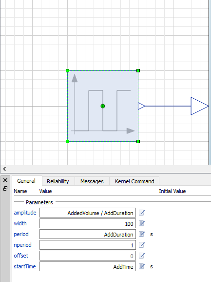
The milk component is simply a pulse from Pulse that has some additional parameters.

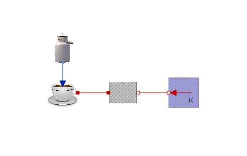
Everything taken together, we now have an additional component in the coffee cooling model:

As it should, this approach gives a similar plot as the first one. The only difference is that the milk is added over a duration of 1 second. As the duration approaches zero, the two approaches would converge.

You could use this approach to fit parameters, using the methodology from the electric kettle example.

Other Cooling Processes

In the model above, we had a very naïve cooling process for our coffee. We assumed it could be described by Newtons law of cooling (which the heat conduction component is based on). In the original thread a paper is linked that goes into detail on how you might expand the a coffee model to include some other forms of cooling.

I will here use a HeatCapacitor component instead of the coffee component to simplify things, but the two should interchangeable. The experiment numbers are in reference to the attached article.

Experiment 1

Experiment 1 can be described using standard components from the Modelica.Thermal.HeatTransfer package. The pot will be HeatCapacitor component, the ambient temperature will be modeled using FixedTemperature and the convection is modeled using a ThermalConductor, which follows Newtons law of cooling.

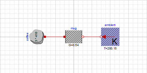
The G parameter in the ThermalConductor is equivalent to the k parameter they use. From what I could tell, the paper did not include any measurement of the heat capacitance or ambient temperature so I went with 3 dl of water and 20 degrees Celsius. However, both of these would probably need to be higher to fit their experimental data.

Experiment 2

To create experiment 2 I first duplicated experiment 1 by selecting it and pressing Ctrl+D, you can also right click and select Duplicate. Experiment 2 requires a component like the ThermalConductor but one that has an exponent that causes nonlinear behaviour in the heat flow. No such component exist in the Modelica Standard Library, but we can easily create one. I created a new component to be used in experiment 2 by dragging the normal ThermalConductor into Experiment2.

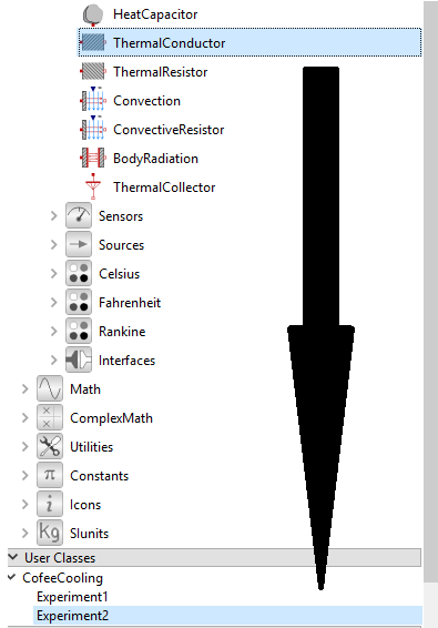
And gave it a new name, "ArbitraryExponentConductor"

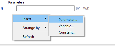
Now I had to modify it to use the exponent. After opening the new component I first added a new parameter by right clicking the parameter view and and selecting Insert > Parameter

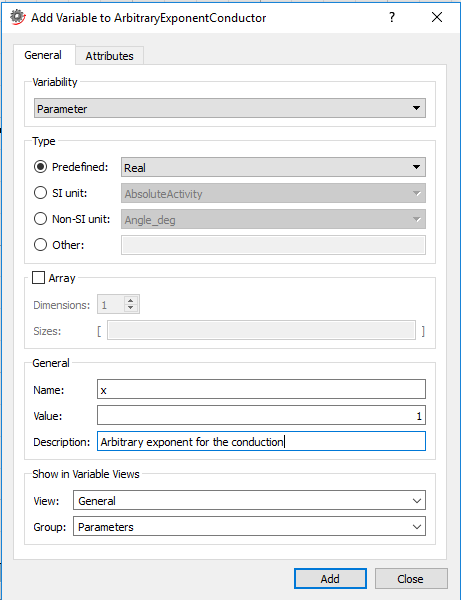
I used the name x as in the paper and used type Real.

Now I had to modify the equations so I went into the Modelica Text View (Ctrl+3) and changed the line:

 Q_flow = G * dT;

to

Q_flow = G * dT ^ x;

dT corresponds to the temperature difference (tc-ts) in the paper.

Going back into Experiment 2, I changed the normal ThermalConductor by right clicking it and selected Change Type. In the dialog, I gave the name of the new type (CofeeCooling.Experiment2.ArbitraryExponentConductor). You can also drag the component from the component browser directly into the field.

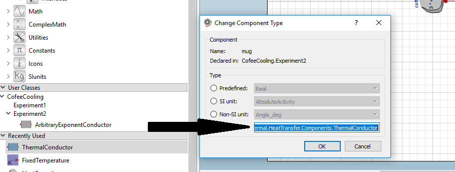
or of course, delete the component, drag the new one in and make new connections.

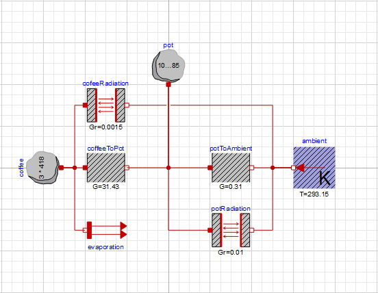
Experiment 3

For experiment 3, you need to add a some more stuff. Start by douplicating experiment 1. Connect the ThermalConductor to a new HeatCapacitor instead of the FixtedTemperature. That heat capacitor will be the pot, while the original one will be the coffee. The first ThermalConductor then represents equation 1 in the paper, transfer of heat from coffee to the pot. Add another ThermalConductor and connect it between the pot and the FixedTemperature to represent equation 5. Also add two BodyRadiation components and connect them from each capacitor to the FixedTemperature. These will represent all the radition effects described. They are bidirectional so they represent two equations each (3,4 and 6,7). For evaporation, I created a custom component which is described by the equation

  port.Q_flow = k * port.T;

Where k is the product of the P, l and v parameters described in the paper. You could add individual parameters for each of them instead, as described in the text for experiment 2.

Connect the evaporation to the coffee capacitor.

The 4:th experiment is much like the the 3:d one. I modified the evaporation component to have the equation

  port.Q_flow = k * port.T ^ z;

Summary & Simulation

Okey, so that was the how. Now we want to use this model to draw conclusions. I'll use the simplest model here and encourage you to try out the more advanced models yourselves.

Say we want to drink our coffee in 2 minutes, starting from 80°C. Everyone knows that the optimal coffee drinking temperature is 72.34°C. When should we add our milk to get there in 2 minutes?

We can do a parametric simulation in Mathematica to try out two different timings:

addTimes = {0, 110};
sim = WSMSimulate["CoffeeAndMilk.Scenarios.Approach1", WSMParameterValues -> {"AddTime" -> addTimes}];

In the plot, I will add a point that is the optimum temperature at time = 120s. I'll also use a trick to get some nice legends to better understand which curve corresponds to which:

WSMPlot[sim, "coffee.T",
 PlotRange -> {{60, 180}, {70, 80}},
 Epilog -> Point[{120, 72.34}],
 PlotLegends -> Map["Add time = " <> ToString[#] &, addTimes]
 ]

This produces the following plot:

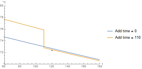
So close. But we can't give up just now. Let us adjust the timing a bit and add the milk right before we want to drink the coffee:

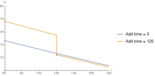
That just about does it I'd say.

Attachments:

CoffeeAndMilk.mo