Introduction
This document discusses concrete algorithms for two different approaches of generation of mandala images, [1]: direct construction with graphics primitives, and use of machine learning algorithms.
In the experiments described in this document better results were obtained with the direct algorithms. The direct algorithms were made for the Mathematica StackExchange question "Code that generates a mandala", [3].
The main goals of this document are:
to show some pretty images exploiting symmetry and multiplicity,
to provide an illustrative example of comparing dimension reduction methods,
to give a set-up for further discussions and investigations on mandala creation with machine learning algorithms.
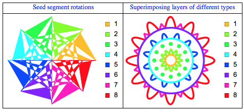
Two direct construction algorithms are given: one uses "seed" segment rotations, the other superimposing of layers of different types. The following plots show the order in which different mandala parts are created with each of the algorithms.
In this document we use several algorithms for dimension reduction applied to collections of images following the procedure described in [4,5]. We are going to show that with Non-Negative Matrix Factorization (NNMF) we can use mandalas made with the seed segment rotation algorithm to extract layer types and superimpose them to make colored mandalas. Using the same approach with Singular Value Decomposition (SVD) or Independent Component Analysis (ICA) does not produce good layers and the superimposition produces more "watered-down", less diverse mandalas.
From a more general perspective this document compares the statistical approach of "trying to see without looking" with the "direct simulation" approach. Another perspective is the creation of "design spaces"; see [6].
The idea of using machine learning algorithms is appealing because there is no need to make the mental effort of understanding, discerning, approximating, and programming the principles of mandala creation. We can "just" use a large collection of mandala images and generate new ones using the "internal knowledge" data of machine learning algorithms. For example, a Neural network system like Deep Dream, [2], might be made to dream of mandalas.
Direct algorithms for mandala generation
In this section we present two different algorithms for generating mandalas. The first sees a mandala as being generated by rotation of a "seed" segment. The second sees a mandala as being generated by different component layers. For other approaches see [3].
The request of [3] is for generation of mandalas for coloring by hand. That is why the mandala generation algorithms are in the grayscale space. Coloring the generated mandala images is a secondary task.
By seed segment rotations
One way to come up with mandalas is to generate a segment and then by appropriate number of rotations to produce a "mandala".
Here is a function and an example of random segment (seed) generation:
Clear[MakeSeedSegment]
MakeSeedSegment[radius_, angle_, n_Integer: 10, connectingFunc_: Polygon, keepGridPoints_: False] :=
  Block[{t},
   t = Table[
     Line[{radius*r*{Cos[angle], Sin[angle]}, {radius*r, 0}}], {r, 0, 1, 1/n}];
   Join[If[TrueQ[keepGridPoints], t, {}], {GrayLevel[0.25],
     connectingFunc@RandomSample[Flatten[t /. Line[{x_, y_}] :> {x, y}, 1]]}]
   ];

seed = MakeSeedSegment[10, Pi/12, 10];
Graphics[seed, Frame -> True]
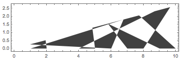
This function can make a seed segment symmetric:
Clear[MakeSymmetric]
MakeSymmetric[seed_] := {seed,
   GeometricTransformation[seed, ReflectionTransform[{0, 1}]]};

seed = MakeSymmetric[seed];
Graphics[seed, Frame -> True]
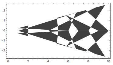
Using a seed we can generate mandalas with different specification signatures:
Clear[MakeMandala]
MakeMandala[opts : OptionsPattern[]] :=
  MakeMandala[
   MakeSymmetric[
    MakeSeedSegment[20, Pi/12, 12,
     RandomChoice[{Line, Polygon, BezierCurve,
       FilledCurve[BezierCurve[#]] &}], False]], Pi/6, opts];

MakeMandala[seed_, angle_?NumericQ, opts : OptionsPattern[]] :=
  Graphics[GeometricTransformation[seed,
    Table[RotationMatrix[a], {a, 0, 2 Pi - angle, angle}]], opts];
This code randomly selects symmetricity and seed generation parameters (number of concentric circles, angles):
SeedRandom[6567]
n = 12;
Multicolumn@
 MapThread[
  Image@If[#1,
     MakeMandala[MakeSeedSegment[10, #2, #3], #2],
     MakeMandala[
      MakeSymmetric[MakeSeedSegment[10, #2, #3, #4, False]], 2 #2]
     ] &, {RandomChoice[{False, True}, n],
   RandomChoice[{Pi/7, Pi/8, Pi/6}, n],
   RandomInteger[{8, 14}, n],
   RandomChoice[{Line, Polygon, BezierCurve,
     FilledCurve[BezierCurve[#]] &}, n]}]
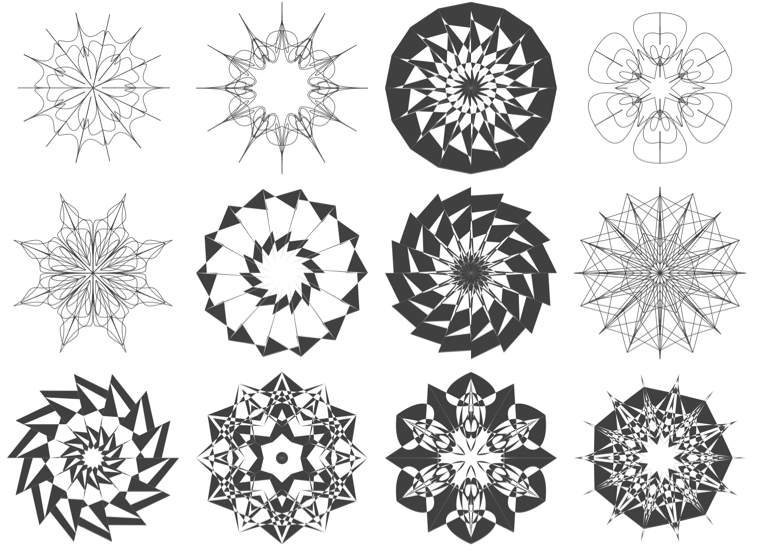
Here is a more concise way to generate symmetric segment mandalas:
Multicolumn[Table[Image@MakeMandala[], {12}], 5]
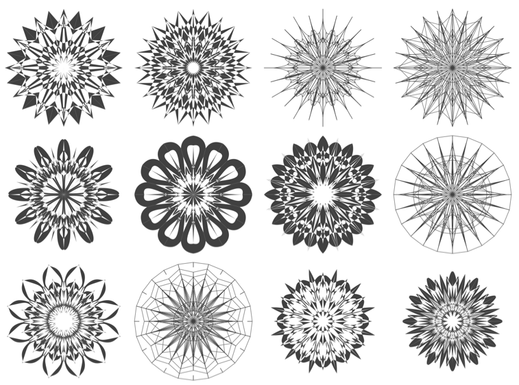
Note that with this approach the programming of the mandala coloring is not that trivial -- weighted blending of colorized mandalas is the easiest thing to do. (Shown below.)
By layer types
This approach was given by Simon Woods in [3].
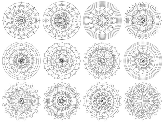
For this one I've defined three types of layer, a flower, a simple circle and a ring of small circles. You could add more for greater variety.
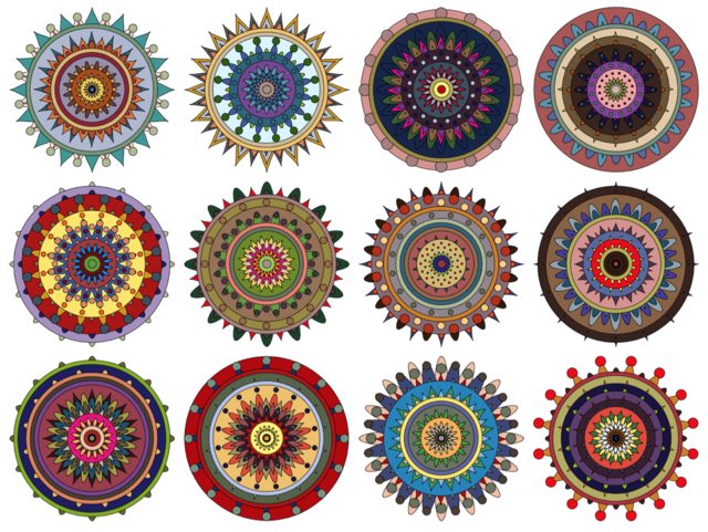
The coloring approach with image blending given below did not work well for this algorithm, so I modified the original code in order to produce colored mandalas.
ClearAll[LayerFlower, LayerDisk, LayerSpots, MandalaByLayers]

LayerFlower[n_, a_, r_, colorSchemeInd_Integer] :=
  Module[{b = RandomChoice[{-1/(2 n), 0}]}, {If[
     colorSchemeInd == 0, White,
     RandomChoice[ColorData[colorSchemeInd, "ColorList"]]],
    Cases[ParametricPlot[
      r (a + Cos[n t])/(a + 1) {Cos[t + b Sin[2 n t]],
        Sin[t + b Sin[2 n t]]}, {t, 0, 2 Pi}],
     l_Line :> FilledCurve[l], -1]}];

LayerDisk[_, _, r_,
   colorSchemeInd_Integer] := {If[colorSchemeInd == 0, White,
    RandomChoice[ColorData[colorSchemeInd, "ColorList"]]],
   Disk[{0, 0}, r]};

LayerSpots[n_, a_, r_,
   colorSchemeInd_Integer] := {If[colorSchemeInd == 0, White,
    RandomChoice[ColorData[colorSchemeInd, "ColorList"]]],
   Translate[Disk[{0, 0}, r a/(4 n)], r CirclePoints[n]]};

MandalaByLayers[n_, m_, coloring : (False | True) : False,
   opts : OptionsPattern[]] :=
  Graphics[{EdgeForm[Black], White,
    Table[RandomChoice[{3, 2, 1} -> {LayerFlower, LayerDisk,
          LayerSpots}][n, RandomReal[{3, 5}], i,
       If[coloring, RandomInteger[{1, 17}], 0]]~Rotate~(Pi i/n), {i,
      m, 1, -1}]}, opts];
Here are black-and-white mandala images.
SeedRandom[6567]
ImageCollage[Table[Image@MandalaByLayers[16, 20], {12}], Background -> White, ImagePadding -> 3, ImageSize -> 1200]
Here are some colored mandalas. (Which make me think more of Viking and Native American art than mandalas.)
ImageCollage[Table[Image@MandalaByLayers[16, 20, True], {12}], Background -> White, ImagePadding -> 3, ImageSize -> 1200]
Training data
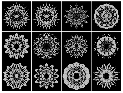
Images by direct generation
iSize = 400;

SeedRandom[6567]
AbsoluteTiming[
 mandalaImages =
   Table[Image[
     MakeMandala[
      MakeSymmetric@
       MakeSeedSegment[10, Pi/12, 12, RandomChoice[{Polygon, FilledCurve[BezierCurve[#]] &}]], Pi/6],
     ImageSize -> {iSize, iSize}, ColorSpace -> "Grayscale"], {300}];
 ]

(* {39.31, Null} *)

ImageCollage[ColorNegate /@ RandomSample[mandalaImages, 12], Background -> White, ImagePadding -> 3, ImageSize -> 400]
External image data
See the section "Using World Wide Web images".
Direct blending
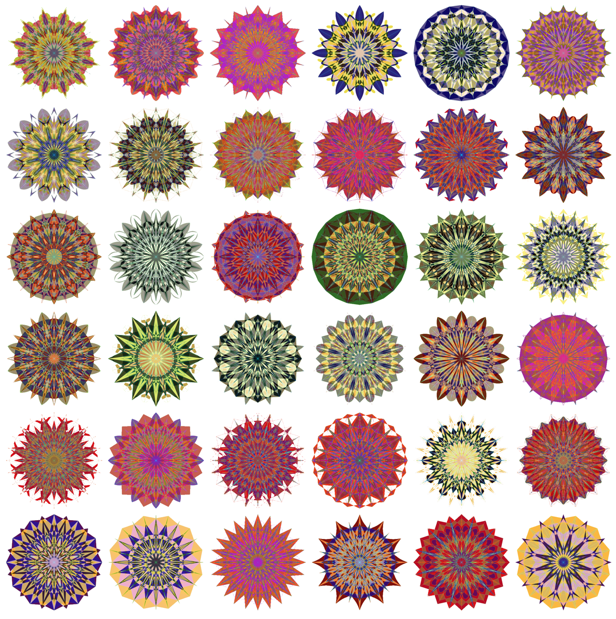
The most interesting results are obtained with the image blending procedure coded below over mandala images generated with the seed segment rotation algorithm.
SeedRandom[3488]
directBlendingImages = Table[
   RemoveBackground@
    ImageAdjust[
     Blend[Colorize[#,
         ColorFunction ->
          RandomChoice[{"IslandColors", "FruitPunchColors",
            "AvocadoColors", "Rainbow"}]] & /@
       RandomChoice[mandalaImages, 4], RandomReal[1, 4]]], {36}];

ImageCollage[directBlendingImages, Background -> White, ImagePadding -> 3, ImageSize -> 1200]
Dimension reduction algorithms application
In this section we are going to apply the dimension reduction algorithms Singular Value Decomposition (SVD), Independent Component Analysis (ICA), and Non-Negative Matrix Factorization (NNMF) to a linear vector space representation (a matrix) of an image dataset. In the next section we use the bases generated by those algorithms to make mandala images. We are going to use the packages [7,8] for ICA and NNMF respectively.
Import["https://raw.githubusercontent.com/antononcube/MathematicaForPrediction/master/IndependentComponentAnalysis.m"]
Import["https://raw.githubusercontent.com/antononcube/MathematicaForPrediction/master/NonNegativeMatrixFactorization.m"]
Linear vector space representation
The linear vector space representation of the images is simple -- each image is flattened to a vector (row-wise), and the image vectors are put into a matrix.
mandalaMat = Flatten@*ImageData@*ColorNegate /@ mandalaImages;
Dimensions[mandalaMat]

(* {300, 160000} *)
Re-factoring and basis images
The following code re-factors the images matrix with SVD, ICA, and NNMF and extracts the basis images.
AbsoluteTiming[
 svdRes = SingularValueDecomposition[mandalaMat, 20];
]
(* {5.1123, Null} *)

svdBasisImages = Map[ImageAdjust@Image@Partition[#, iSize] &, Transpose@svdRes[[3]]];

AbsoluteTiming[
 icaRes =
   IndependentComponentAnalysis[Transpose[mandalaMat], 20,
    PrecisionGoal -> 4, "MaxSteps" -> 100];
]
(* {23.41, Null} *)

icaBasisImages = Map[ImageAdjust@Image@Partition[#, iSize] &, Transpose[icaRes[[1]]]];

SeedRandom[452992]
AbsoluteTiming[
 nnmfRes =
   GDCLS[mandalaMat, 20, PrecisionGoal -> 4,
    "MaxSteps" -> 20, "RegularizationParameter" -> 0.1];
 ]
(* {233.209, Null} *)

nnmfBasisImages = Map[ImageAdjust@Image@Partition[#, iSize] &, nnmfRes[[2]]];
Bases
Let us visualize the bases derived with the matrix factorization methods.
Grid[{{"SVD", "ICA", "NNMF"},
      Map[ImageCollage[#, Automatic, {400, 500},
        Background -> LightBlue, ImagePadding -> 5, ImageSize -> 350] &,
      {svdBasisImages, icaBasisImages, nnmfBasisImages}]
     }, Dividers -> All]
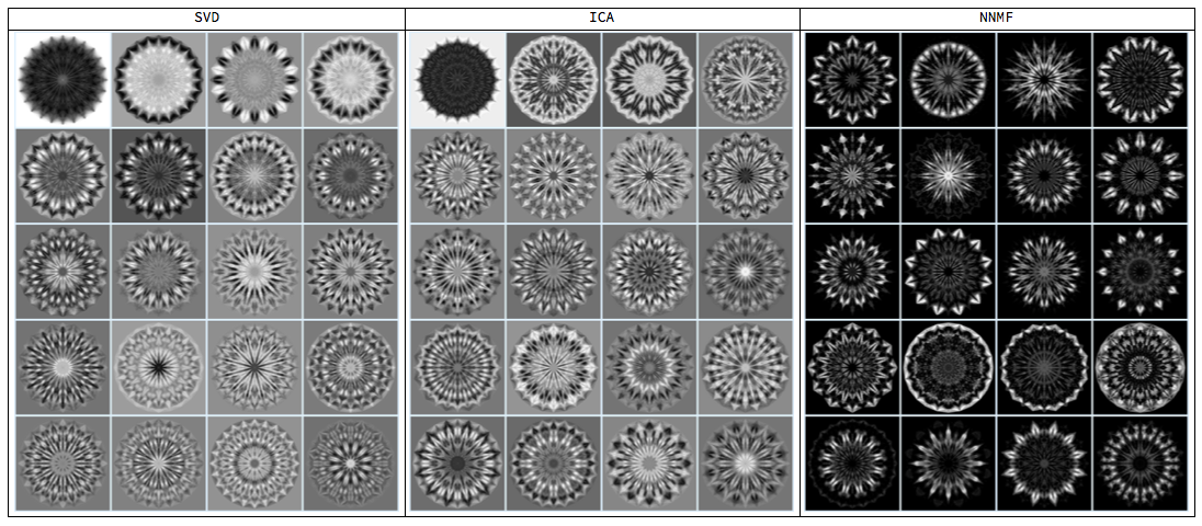
Here are some observations for the bases.
The SVD basis has an average mandala image as its first vector and the other vectors are "differences" to be added to that first vector.
The SVD and ICA bases are structured similarly. That is because ICA and SVD are both based on orthogonality -- ICA factorization uses an orthogonality criteria based on Gaussian noise properties (which is more relaxed than SVD's standard orthogonality criteria.)
As expected, the NNMF basis images have black background because of the enforced non-negativity. (Black corresponds to 0, white to 1.)
Compared to the SVD and ICA bases the images of the NNMF basis are structured in a radial manner. This can be demonstrated using image binarization.
Grid[{{"SVD", "ICA", "NNMF"}, Map[ImageCollage[Binarize[#, 0.5] & /@ #, Automatic, {400, 500}, Background -> LightBlue, ImagePadding -> 5, ImageSize -> 350] &, {svdBasisImages, icaBasisImages, nnmfBasisImages}] }, Dividers -> All]
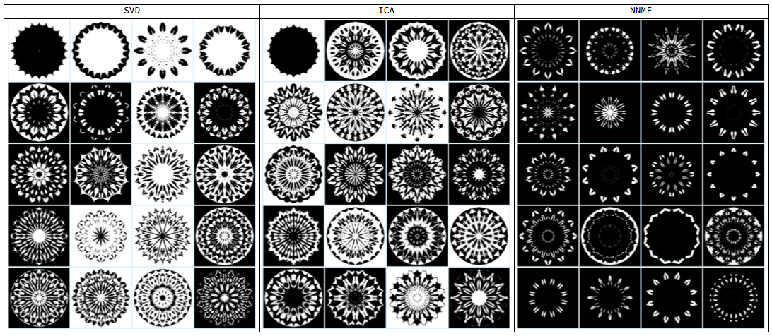
We can see that binarizing the NNMF basis images shows them as mandala layers. In other words, using NNMF we can convert the mandalas of the seed segment rotation algorithm into mandalas generated by an algorithm that superimposes layers of different types.
Blending with image bases samples
In this section we just show different blending images using the SVD, ICA, and NNMF bases.
Blending function definition
ClearAll[MandalaImageBlending]
Options[MandalaImageBlending] = {"BaseImage" -> {}, "BaseImageWeight" -> Automatic, "PostBlendingFunction" -> (RemoveBackground@*ImageAdjust)};
MandalaImageBlending[basisImages_, nSample_Integer: 4, n_Integer: 12, opts : OptionsPattern[]] :=
  Block[{baseImage, baseImageWeight, postBlendingFunc, sImgs, sImgWeights},
   baseImage = OptionValue["BaseImage"];
   baseImageWeight = OptionValue["BaseImageWeight"];
   postBlendingFunc = OptionValue["PostBlendingFunction"];
   Table[(
     sImgs =
      Flatten@Join[{baseImage}, RandomSample[basisImages, nSample]];
     If[NumericQ[baseImageWeight] && ImageQ[baseImage],
      sImgWeights =
       Join[{baseImageWeight}, RandomReal[1, Length[sImgs] - 1]],
      sImgWeights = RandomReal[1, Length[sImgs]]
      ];
     postBlendingFunc@
      Blend[Colorize[#,
          DeleteCases[{opts}, ("BaseImage" -> _) | ("BaseImageWeight" -> _) | ("PostBlendingFunction" -> _)],
          ColorFunction ->
           RandomChoice[{"IslandColors", "FruitPunchColors",
             "AvocadoColors", "Rainbow"}]] & /@ sImgs,
       sImgWeights]), {n}]
   ];
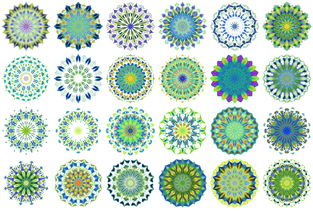
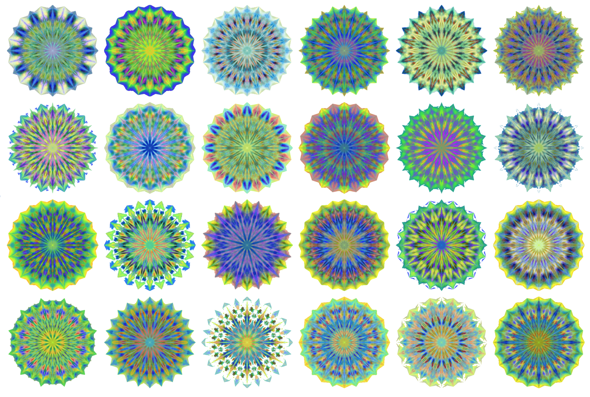
SVD image basis blending
SeedRandom[17643]
svdBlendedImages = MandalaImageBlending[Rest@svdBasisImages, 4, 24];
ImageCollage[svdBlendedImages, Background -> White, ImagePadding -> 3, ImageSize -> 1200]
SeedRandom[17643]
svdBlendedImages = MandalaImageBlending[Rest@svdBasisImages, 4, 24, "BaseImage" -> First[svdBasisImages], "BaseImageWeight" -> 0.5];
ImageCollage[svdBlendedImages, Background -> White, ImagePadding -> 3, ImageSize -> 1200]
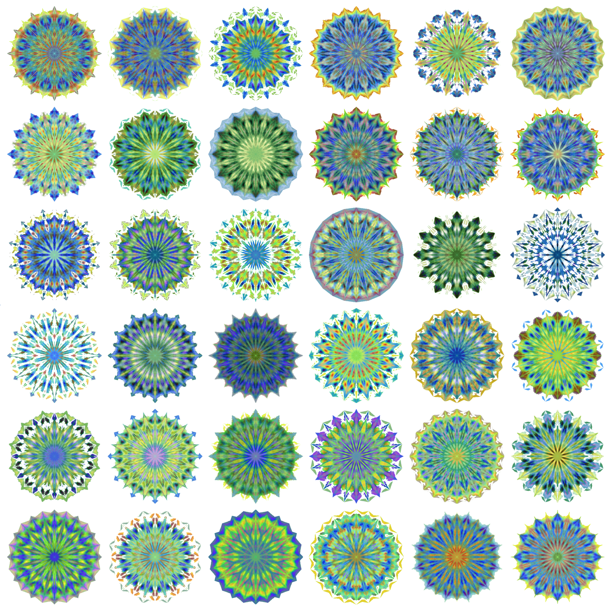
ICA image basis blending
SeedRandom[17643]
icaBlendedImages = MandalaImageBlending[Rest[icaBasisImages], 4, 36, "BaseImage" -> First[icaBasisImages], "BaseImageWeight" -> Automatic];
ImageCollage[icaBlendedImages, Background -> White, ImagePadding -> 3, ImageSize -> 1200]
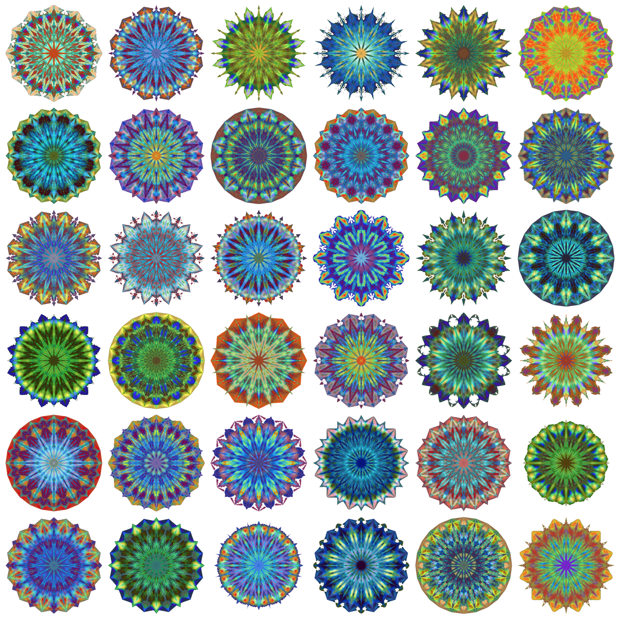
NNMF image basis blending
SeedRandom[17643]
nnmfBlendedImages = MandalaImageBlending[nnmfBasisImages, 4, 36];
ImageCollage[nnmfBlendedImages, Background -> White, ImagePadding -> 3, ImageSize -> 1200]
Using World Wide Web images
A natural question to ask is:
What would be the outcomes of the above procedures to mandala images found in the World Wide Web (WWW) ?
Those WWW images are most likely man made or curated.
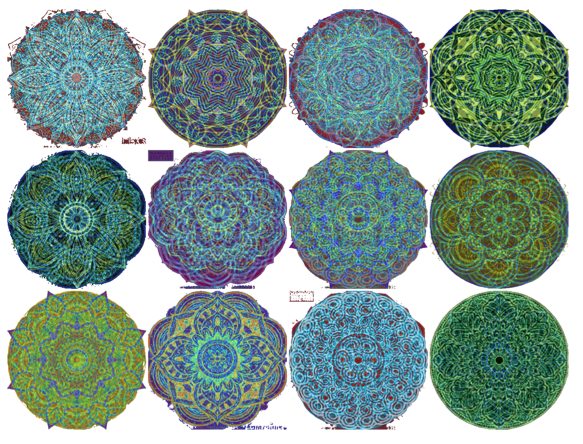
The short answer is that the results are not that good. Better results might be obtained using a larger set of WWW images (than just 100 in the experiment results shown below.)
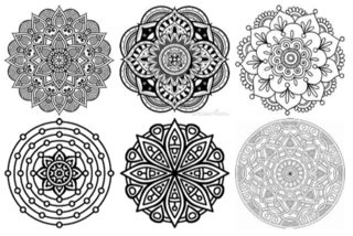
Here is a sample from the WWW mandala images:
Here are the results obtained with NNMF basis:
Future plans
My other motivation for writing this document is to set up a basis for further investigations and discussions on the following topics.
Having a large image database of "real world", human made mandalas.
Utilization of Neural Network algorithms to mandala creation.
Utilization of Cellular Automata to mandala generation.
Investigate mandala morphing and animations.
Making a domain specific language of specifications for mandala creation and modification.
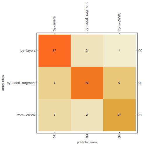
The idea of using machine learning algorithms for mandala image generation was further supported by an image classifier that recognizes fairly well (suitable normalized) mandala images obtained in different ways:
References
[1] Wikipedia entry, Mandala, https://en.wikipedia.org/wiki/Mandala .
[2] Wikipedia entry, DeepDream, https://en.wikipedia.org/wiki/DeepDream .
[3] "Code that generates a mandala", Mathematica StackExchange, http://mathematica.stackexchange.com/q/136974 .
[4] Anton Antonov, "Comparison of PCA and NNMF over image de-noising", (2016), MathematicaForPrediction at WordPress blog. URL: https://mathematicaforprediction.wordpress.com/2016/05/07/comparison-of-pca-and-nnmf-over-image-de-noising/ .
[5] Anton Antonov, "Handwritten digits recognition by matrix factorization", (2016), MathematicaForPrediction at WordPress blog. URL: https://mathematicaforprediction.wordpress.com/2016/11/12/handwritten-digits-recognition-by-matrix-factorization/ .
[6] Chris Carlson, "Social Exploration of Design Spaces: A Proposal", (2016), Wolfram Technology Conference 2016. URL: http://wac .36f4.edgecastcdn.net/0036F4/pub/www.wolfram.com/technology-conference/2016/SocialExplorationOfDesignSpaces.nb , YouTube: https://www.youtube.com/watch?v=YK2523nfcms .
[7] Anton Antonov, Independent Component Analysis Mathematica package, (2016), source code at [MathematicaForPrediction at GitHub](https://github.com/antononcube/MathematicaForPrediction/), package IndependentComponentAnalysis.m .
[8] Anton Antonov, Implementation of the Non-Negative Matrix Factorization algorithm in Mathematica, (2013), source code at [MathematicaForPrediction at GitHub](https://github.com/antononcube/MathematicaForPrediction/), package NonNegativeMatrixFactorization.m.