Introduction
So here is a simple approach that applies Wolfram Language machine learning functions to a classification problem for finding possible Higgs particles. It uses a labeled data set with 30 numerical physical attributes (things like measured spins, angles, energies, etc.) and with labels being either 'signal' (s) or 'background' (b). The attached notebook runs through a sample analysis in the Wolfram Language: importing the training data, cleaning it up for using it, setting up a neural network, training the network with the data, and finally checking how well the trained neural network does at making predictions. Here is the description of data from the source website at KAGGLE:
Discovery of the long awaited Higgs boson was announced July 4, 2012 and confirmed six months later. 2013 saw a number of prestigious awards, including a Nobel prize. But for physicists, the discovery of a new particle means the beginning of a long and difficult quest to measure its characteristics and determine if it fits the current model of nature.
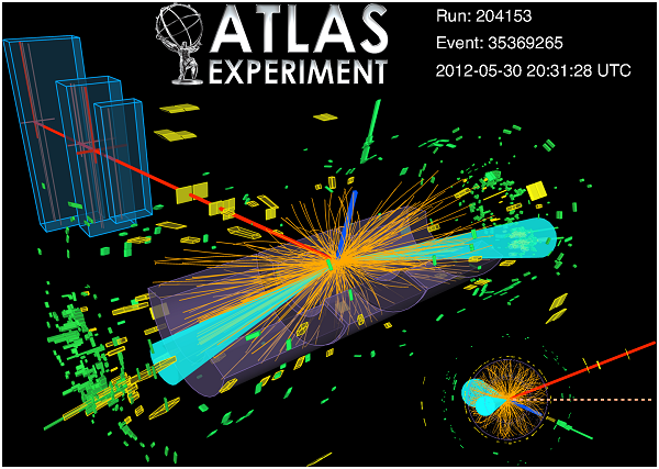
A key property of any particle is how often it decays into other particles. ATLAS is a particle physics experiment taking place at the Large Hadron Collider at CERN that searches for new particles and processes using head-on collisions of protons of extraordinarily high energy. The ATLAS experiment has recently observed a signal of the Higgs boson decaying into two tau particles, but this decay is a small signal buried in background noise.
The goal of the Higgs Boson Machine Learning Challenge is to explore the potential of advanced machine learning methods to improve the discovery significance of the experiment. No knowledge of particle physics is required. Using simulated data with features characterizing events detected by ATLAS, your task is to classify events into "tau tau decay of a Higgs boson" versus "background."
The winning method may eventually be applied to real data and the winners may be invited to CERN to discuss their results with high energy physicists.
References and sources
Training data
Import the training data:
training = Import["D:\\machinelearning\\higgs\\training\\training.csv", "Data"];
Dimensions[training]
{250001, 33}
Look at the data fields (they are described in the pdf link above). "EventId" should not be used as part of the training, since it has no predictive value. The last column "Label" is the classification (s=signal, b=background)
training[[1]]
{"EventId", "DER_mass_MMC", "DER_mass_transverse_met_lep", \ "DER_mass_vis", "DER_pt_h", "DER_deltaeta_jet_jet", \ "DER_mass_jet_jet", "DER_prodeta_jet_jet", "DER_deltar_tau_lep", \ "DER_pt_tot", "DER_sum_pt", "DER_pt_ratio_lep_tau", \ "DER_met_phi_centrality", "DER_lep_eta_centrality", "PRI_tau_pt", \ "PRI_tau_eta", "PRI_tau_phi", "PRI_lep_pt", "PRI_lep_eta", \ "PRI_lep_phi", "PRI_met", "PRI_met_phi", "PRI_met_sumet", \ "PRI_jet_num", "PRI_jet_leading_pt", "PRI_jet_leading_eta", \ "PRI_jet_leading_phi", "PRI_jet_subleading_pt", \ "PRI_jet_subleading_eta", "PRI_jet_subleading_phi", "PRI_jet_all_pt", \ "Weight", "Label"}
Sample vector:
training[[2]]
{100000, 138.47, 51.655, 97.827, 27.98, 0.91, 124.711, 2.666, 3.064, \ 41.928, 197.76, 1.582, 1.396, 0.2, 32.638, 1.017, 0.381, 51.626, \ 2.273, -2.414, 16.824, -0.277, 258.733, 2, 67.435, 2.15, 0.444, \ 46.062, 1.24, -2.475, 113.497, 0.00265331, "s"}
Set up a simple neural network (this can be tinkered with to improve the results):
net=NetInitialize[
NetChain[{
LinearLayer[3000],Ramp,LinearLayer[3000],Ramp,LinearLayer[2],SoftmaxLayer[]
},
"Input"->{30},
"Output"->NetDecoder[{"Class",{"b","s"}}]
]]

Set up the training data:
data = Map[Take[#, {2, 31}] -> Last[#] &, Drop[training, 1]];
Numerical vectors that each point to a classification (s or b):
RandomSample[data, 3]
{{87.06, 23.069, 67.711, 162.488, -999., -999., -999., 0.903, 4.245, 318.43, 0.523, 0.839, -999., 105.019, -0.404, 1.612, 54.943, -0.898, 0.855, 13.541, 1.729, 409.232, 1, 158.469, -1.363, -1.762, -999., -999., -999., 158.469} -> "b", {163.658, 55.559, 116.84, 50.019, -999., -999., -999., 2.855, 38.623, 130.132, 0.906, 1.359, -999., 51.993, 0.36, 2.142, 47.112, -0.932, -1.596, 22.782, 2.663, 191.557, 1, 31.026, -2.333, 0.739, -999., -999., -999., 31.026} -> "b", {100.248, 27.109, 60.729, 132.094, -999., -999., -999., 1.405, 10.063, 218.474, 0.541, 1.414, -999., 62.519, -0.401, -1.974, 33.817, -0.893, -0.657, 54.857, -1.298, 396.228, 1, 122.137, -2.369, 1.689, -999., -999., -999., 122.137} -> "s"}
Training
Length[data]
250000
{tdata,vdata}=TakeDrop[data,240000];
result=NetTrain[net,tdata,TargetDevice->"GPU",ValidationSet->Scaled[0.1],MaxTrainingRounds->1000]

DumpSave["D:\\machinelearning\\higgs\\higgs.mx", result];
Testing
This is the test data (unlabeled):
test = Import["D:\\machinelearning\\higgs\\test\\test.csv", "Data"];
Extract the validation data:
validate = Map[Take[#, {2, 31}] &, Drop[test, 1]];
Predictions made on the unlabeled data:
result /@ RandomSample[validate, 5]
{"b", "b", "s", "b", "b"}
Sample from the labeled data and compute classifier statistics:
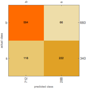
cm = ClassifierMeasurements[result, RandomSample[vdata, 1000]]

cm["Accuracy"]
0.846
Plot the confusion matrix:
cm["ConfusionMatrixPlot"]
