Here is something that I do in my lectures regarding the coffee cooling problem. I use just standard Mathematica and a rather simple approach based on Newton's law for cooling. See also a related System Modeler post.
Newton's Law of Cooling
When Newton described the cooling for an object, he used the simple assumption that the change of the temperature of an object is proportional to the temperature difference of the environment and the object.

Here Temp(t) is the temperature of the object and TU is the temperature of the environment, e.g. the ambient air. The coefficient $\kappa$ indicates how fast the adaptation to the outside temperature takes place.
In Mathematica it looks like this:
sols = DSolve[{D[Temp[t], t] == -\[Kappa] (Temp[t] - TU), Temp[0] == T0}, Temp, t]
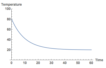
Here we assume that the starting temperature is T0. If we assume the starting temperature to be 80 degrees C and the air temperature to be 20 degrees C, and $\kappa=0.1$ we obtain the following plot.
Plot[Temp[t] /. sols /. {\[Kappa] -> 0.1, TU -> 20, T0 -> 80}, {t, 0, 60}, PlotRange -> {All, {0, 100}},
AxesLabel -> {"Time", "Temperature"}, LabelStyle -> Directive[Bold, Medium]]
In fact, if we had data we could determine the value for $\kappa$ from experiments.
When do I put the milk in my coffee?
So here's the question. If I am in a hurry in the morning and need to catch a bus. I love my coffee but do not want to burn my lips. When do I pour the cold milk in? As early on as I can or just before I need to leave the house?
We can easily model the adding of milk to some coffee by using the WhenEvent function:
sols = NDSolve[{D[Temp[t], t] == -0.1 (Temp[t] - 20), Temp[0] == 80,
   WhenEvent[t > 1, Temp[t] -> (200. Temp[t] + 50.* 5.)/250.]},
  Temp, {t, 0, 30}]
it uses a simplified version of the law that governs the mixing of fluids (same calorific capacities).

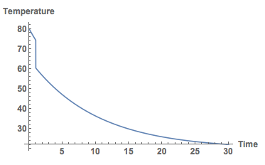
where Tmix is the temperature of the resulting coffee-milk mix, mc and mm are the mass of the coffee and the milk, and Tc and Tm their respective temperatures. Note that the model is not quite correct in the sense that it does not take into consideration that the mass of the content of the mug has changed after the milk is added. First we put the milk in right at the beginning:
sols = NDSolve[{D[Temp[t], t] == -0.1 (Temp[t] - 20), Temp[0] == 80,
WhenEvent[t > 1, Temp[t] -> (200. Temp[t] + 50.* 5.)/250.]},
Temp, {t, 0, 30}]
Here's the graph.
Plot[Temp[t] /. sols, {t, 0, 30}, PlotRange -> All, AxesLabel -> {"Time", "Temperature"}, LabelStyle -> Directive[Bold, Medium]]
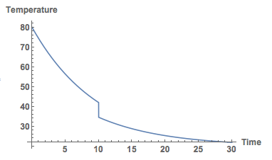
Next we wait for 10 minutes and then pour the milk in:
sols2 = NDSolve[{D[Temp[t], t] == -0.1 (Temp[t] - 20), Temp[0] == 80, WhenEvent[t > 10, Temp[t] -> (200.* Temp[t] + 50.* 5.)/250.]}, Temp, {t, 0, 30}]
Here's the plot:
Plot[Temp[t] /. sols2, {t, 0, 30}, PlotRange -> All, AxesLabel -> {"Time", "Temperature"},
 LabelStyle -> Directive[Bold, Medium]]
If we plot both together we get this:
Show[Plot[Temp[t] /. sols, {t, 0, 30}, PlotRange -> All], Plot[Temp[t] /. sols2, {t, 0, 30}, PlotRange -> All],
AxesLabel -> {"Time", "Temperature"}, LabelStyle -> Directive[Bold, Medium]]
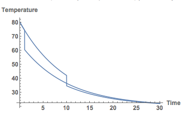
Clearly, I should put my milk in as late as possible. Well, that's the model.
Getting data for our model
Let's get some data with an Arduino and a simple temperature sensor. We use a standard Arduino Uno and wire it like so:
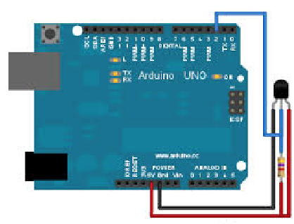
I use a standard Arduino and a Dallas Temperature Sensor. We then need to upload an Arduino C-program, which is called Sketch, to the microcontroller.
#include <OneWire.h>
#include <DallasTemperature.h>

// Data wire is plugged into pin 2 on the Arduino
#define ONE_WIRE_BUS 2

// Setup a oneWire instance to communicate with any OneWire devices
// (not just Maxim/Dallas temperature ICs)
OneWire oneWire(ONE_WIRE_BUS);

// Pass our oneWire reference to Dallas Temperature.
DallasTemperature sensors(&oneWire);

void setup(void)
{
  // start serial port
  Serial.begin(9600);

  // Start up the library
  sensors.begin();
}


void loop(void)
{

  sensors.requestTemperatures(); // Send the command to get temperatures

  Serial.print(sensors.getTempCByIndex(0),4);
  Serial.print(",");
}
The upload is done via the Arduino IDE. (I could do it directly from within Mathematica.)
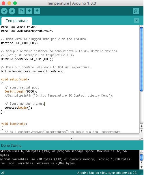
The Arduino is connected via a serial (i.e. USB) cable to the computer. Mathematica can connect to the serial port like so (on a Mac, slightly different on a Windows machine):
myDSTemperature =
 DeviceOpen["Serial", {Quiet[FileNames["tty.usb*", {"/dev"}, Infinity]][[1]], "BaudRate" -> 9600}]
We can then run a ScheduledTask every second:
s = {}; tZero = AbsoluteTime[]; DeviceReadBuffer[myDSTemperature];
RunScheduledTask[
AppendTo[s, {AbsoluteTime[] - tZero, ToExpression@(StringSplit[FromCharacterCode@DeviceReadBuffer[myDSTemperature], ","][[-1]])}], 1]
We can then display the result dynamically:
Dynamic[ListLinePlot[s, PlotRange -> {All, {20, 40}}]]
After that you might want to stop the Scheduled task and close the connection:
RemoveScheduledTask /@ ScheduledTasks[];
DeviceClose[myDSTemperature]
I have attached the measurements I obtained for my experiment. You can load and display it like this:
ClearAll["Global`*"]

data = Import["~/Desktop/temperaturedata_CoffeMilkGood.csv"];
dataclean = Table[Join[{data[[k]][[1 ;; 6]]}, data[[k]][[7 ;; 9]]], {k, 1, Length[data]}];
data2plotearlymilk = Select[Transpose[{dataclean[[All, 1]], dataclean[[All, 3]]/1000.}], #[[2]] > 0 &];
data2plotlatemilk = Select[Transpose[{dataclean[[All, 1]], dataclean[[All, 2]]/1000.}], #[[2]] > 0 &];

DateListPlot[{data2plotearlymilk, data2plotlatemilk}, PlotRange -> {All, {0, 100}}, Joined -> True,
FrameLabel -> {"Time", "Temperature"}, LabelStyle -> Directive[Bold, Medium]]
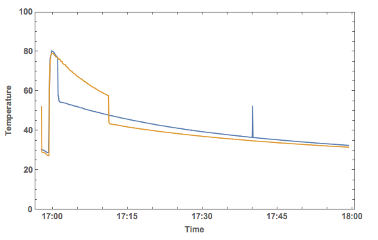
There is clearly one measurement error at the blue curve, but it does appear to show that there is a better chance of not burning my lips if I put the milk in as late as I can.
Note that I have assumed that the air temperature does not change. In fact, I also measured the air temperature when I did the experiment - it is constant as expected.
As I said, I know that this is not really addressing the original question, but when I teach mathematical modelling, I always like showing the students that is quite relevant to compare the models to data.
Cheers,
Marco
 Attachments: