The idea of this thread is from a question raised by
Dongyi Wei, who is a very competitive first tier math olympiad in China. He proposed the following inequality should hold for positive real numbers a, b and c:

He sent this problem to his buddy to seek a solution in terms of elementary and algebraic method, which is very lengthy and tricky. Since I am more engineer than a math athlete, I do not think I can come up with that tricky solution and I just want things "work".
To make the problem easier to describe, I defined two functions for each side of the inequality: f is for the lhs
f[a_, b_, c_] = (1 - a)^2 + (1 - b)^2 + (1 - c)^2;
and g is for the rhs
g[a_, b_, c_] = (1 - a^2) (1 - b^2) c^2/(a b + c)^2 + (1 - b^2) (1 - c^2) a^2/(b c + a)^2 + (1 - c^2) (1 - a^2) b^2/(c a + b)^2;
(It is preferred to use Set instead of SetDelay(:=) in this case)
My first attempt was a simple brutal-force method, I just used
Maximize[{g[a, b, c]/f[a, b, c], a > 0, b > 0, c > 0}, {a, b, c}]
which seemed to take forever to return the expected result, 1. This definitely does not work. Also I realize that I cannot evern visualize f and g because they have three variables and their plot would require the 4th dimension.
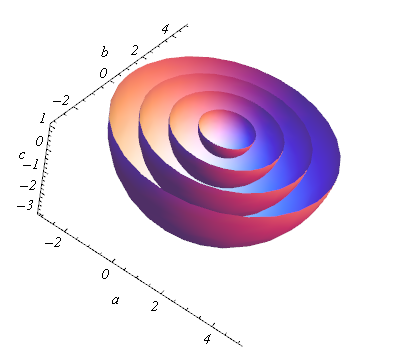
As I read the problem twice, I noticed that if this inequality holds and I gave f[a,b,c] a fixed value, then this value should be the max value of the rhs. Aha! That sounds like I can study this problem by the contours of f and g. Based on the form of the two function f and g, it is easier to find the proper a, b and c for f than for g if a fixed value is given, Actually, f[a, b,c ] == constant yields a standard form for a 2-D sphere. I can quickly parameterize a, b and c here using spherical coordinates: (upper half is removed for demonstration, r is the radius of each sphere)
ParametricPlot3D[
Table[{r*Cos[?] Cos[?] + 1, r*Cos[?] Sin[?] + 1, r*Sin[?] + 1}, {r, 1, 4}], {?, 0, 2 ?}, {?, -?, 0},
AxesLabel -> {a, b, c}, LabelStyle -> {Italic, FontSize -> 15}, Mesh -> None, Boxed -> False]
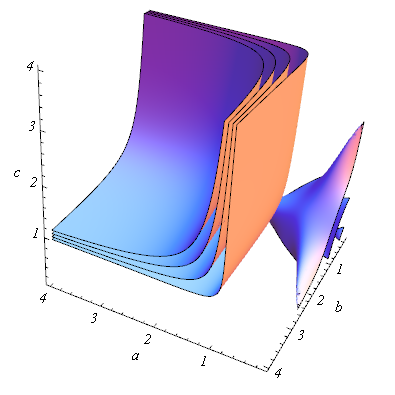
While g is super complicated:
Show[Sequence @@ (ContourPlot3D[
g[a, b, c] == #, {a, 0.1, 4}, {b, 0.1, 4}, {c, 0.1, 4},
AxesLabel -> {a, b, c}, LabelStyle -> {Italic, FontSize -> 15},
Contours -> 3, Mesh -> None, Boxed -> False] & /@ {0.1, 1, 2, 3})
]
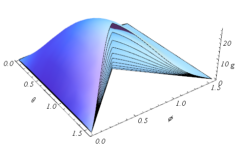
Note that this is still a plot for the contour of f and g in terms of a, b and c. If I plot f against theta and phi, it is just a plane with f = r^2 in the theta-phi-f coordinate. After I set a value for f, it is also required that the values of a, b and c in the rhs must be the same set of a, b and c used in the lhs. Thus I can just use the parameterized a, b and c in the function g, ie. converting
g[a,b,c]
to
g[r*Cos[\[Phi]] Cos[\[Theta]] + 1, r*Cos[\[Phi]] Sin[\[Theta]] + 1, r*Sin[\[Phi]] + 1]
Now I can plot the g against theta and phi with Plot3D as r is set. So what I am looking for now is whether the maximum value of g exceeds r^2, a preset value for f. For some r's (from 0.5 to 5, the step length be 0.5), I can find related surfaces (a quater is removed for demonstration purpose):
Plot3D[Table[ With[{r = r},
g[r*Cos[?] Cos[?] + 1, r*Cos[?] Sin[?] + 1,r*Sin[?] + 1]], {r, 0.5, 5, 0.5}
],
{?, 0, ?/2}, {?, 0, ?/2}, AxesLabel -> {?, ?, "g"}, LabelStyle -> {Italic, FontSize -> 15},
PlotRange -> Full, Mesh -> None,
RegionFunction -> Function[{x, y, z}, ?/4 < Abs[x - ?/2] + Abs[y - ?/4]], Boxed -> False
]
Just for convience, I can define a functional h:
h[r_] = g[r*Cos[\[Phi]] Cos[\[Theta]] + 1, r*Cos[\[Phi]] Sin[\[Theta]] + 1, r*Sin[\[Phi]] + 1]
So the maximum value of each slide of this square dumpling is NMaximize[h,...]. For instance, when r is 2, I have
In[5]:= NMaximize[{Evaluate[h[2]], 0 < \[Theta] < \[Pi]/2, 0 < \[Phi] < \[Pi]/2}, {\[Theta], \[Phi]}]
Out[5]= {4., {\[Theta] -> 0.785398, \[Phi] -> 0.61548}}
I can also tabulate the results for several r's:
In[6]:= Table[
{i, NMaximize[{Evaluate[h[i]], 0 < \[Theta] < \[Pi]/2, 0 < \[Phi] < \[Pi]/2}, {\[Theta], \[Phi]}][[1]]},
{i, 0.5, 5, 0.2}
] // TableForm[#, TableHeadings -> {None, {"r", "g_Max"}}] &
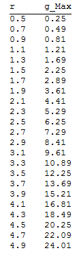
We can see that the maximum value of g is clearly r^2 and Wen's proposal at least is emperically correct.


