Group Abstract Group Abstract

Message Boards Message Boards

[?] Avoid differences between solutions by NDsolve and by OutputResponse?

Dear Members of the of the community I have written a very simple piece of code to dynamically calculate Fourier coefficients of a signal. The code is something like this

f = 60;
h = 6;(*Harmonic number*)

u1[t_] = Sin[2 \[Pi] f t] + 5 Sin[2 \[Pi] 3 f t] + 
  0.8 Cos[2 \[Pi] 6 f t] + 5;
tau = 1/f;m2 = NDSolve[{
    ff1'[t] == u1[t] Cos[2 \[Pi] 6 f t], ff1[t /; t <= 0] == 0.0,
    f2'[t] == ff1'[t - tau], f2[t /; t <= 0] == 0}, {ff1[t], 
    f2[t]}, {t, 0, 3 tau}];
Plot[Evaluate[{2 f (ff1[t] - f2[t])} /. m2], {t, 0, 3 tau}, 
 PlotRange -> All]

For a signal

u1[t_] = Sin[2 \[Pi] f t] + 5 Sin[2 \[Pi] 3 f t] + 
   0.8 Cos[2 \[Pi] 6 f t] + 5;

The plot would be

enter image description here

After a transient the output converges to 0.8, that is the coefficient of the sixth harmonic in u[t]. I have try the same defining a model by StateSpaceModel and solving with OutputResponse.

m1 = StateSpaceModel[{ff1'[t] == signal[t] Cos[2 \[Pi] h f t], 
    f2'[t] == ff1'[t - tau]}, {ff1[t], 
    f2[t]}, {signal[t]}, {2 f (ff1[t] - f2[t])}, t];
y1 = OutputResponse[m1, u1[t], {t, 0, 3 tau}];
Plot[y1, {t, 0, 3 tau}]

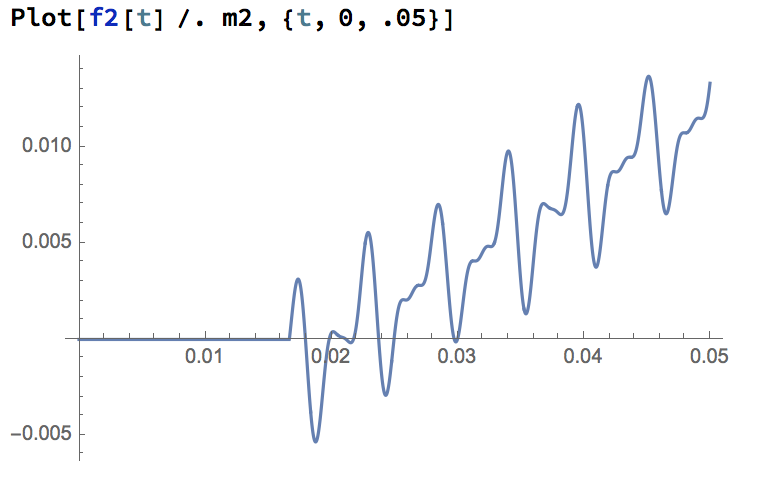
In such a case the output is .

enter image description here

It seems to me that both models are equivalent and should produce same results but they don't!.
Could anybody give a hint on what I am doing wrong?

Cheers Jesus Rico

2 Replies

Neil,

Thanks for you suggestion. You are right, it has to do with the delay. There are two way to delay a state variable 1) x[t-tau] or 2) SystemModelDelay[tau] x[t]. They are equivalent according to the documentation but in this case they are not. I found that the following code it does work

f = 60;
h = 3;(*Harmonic number*)

u1[t_] = Sin[2 \[Pi] f t] + 5 Cos[2 \[Pi] 3 f t] + 
  0.8 Cos[2 \[Pi] 6 f t] + 3;
tau = 1/f;
m1 = StateSpaceModel[{ff1'[t] == signal[t] Cos[2 \[Pi] h f t], 
   f2'[t] ==   SystemsModelDelay[tau] ff1'[t]}, {ff1[t], 
   f2[t]}, {signal[t]}, {2 f (ff1[t] - f2[t])}, t]
y1 = OutputResponse[m1, u1[t], {t, 0, 3 tau}];
Plot[y1, {t, 0, 3 tau}]

enter image description here

Interestingly, the resulting state space model is in Descriptor Form

enter image description here

I am going on to my control books to properly understand why!

Cheers Jesús

POSTED BY: Neil Singer
Reply to this discussion
Community posts can be styled and formatted using the Markdown syntax.
Reply Preview
Attachments
Remove
or Discard