Message Boards Message Boards

[?] Avoid differences between solutions by NDsolve and by OutputResponse?

Dear Members of the of the community I have written a very simple piece of code to dynamically calculate Fourier coefficients of a signal. The code is something like this

f = 60;
h = 6;(*Harmonic number*)

u1[t_] = Sin[2 \[Pi] f t] + 5 Sin[2 \[Pi] 3 f t] + 
  0.8 Cos[2 \[Pi] 6 f t] + 5;
tau = 1/f;m2 = NDSolve[{
    ff1'[t] == u1[t] Cos[2 \[Pi] 6 f t], ff1[t /; t <= 0] == 0.0,
    f2'[t] == ff1'[t - tau], f2[t /; t <= 0] == 0}, {ff1[t], 
    f2[t]}, {t, 0, 3 tau}];
Plot[Evaluate[{2 f (ff1[t] - f2[t])} /. m2], {t, 0, 3 tau}, 
 PlotRange -> All]

For a signal

u1[t_] = Sin[2 \[Pi] f t] + 5 Sin[2 \[Pi] 3 f t] + 
   0.8 Cos[2 \[Pi] 6 f t] + 5;

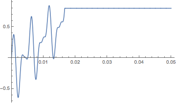
The plot would be
enter image description here

After a transient the output converges to 0.8, that is the coefficient of the sixth harmonic in u[t]. I have try the same defining a model by StateSpaceModel and solving with OutputResponse.

m1 = StateSpaceModel[{ff1'[t] == signal[t] Cos[2 \[Pi] h f t], 
    f2'[t] == ff1'[t - tau]}, {ff1[t], 
    f2[t]}, {signal[t]}, {2 f (ff1[t] - f2[t])}, t];
y1 = OutputResponse[m1, u1[t], {t, 0, 3 tau}];
Plot[y1, {t, 0, 3 tau}]

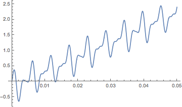
In such a case the output is .
enter image description here

It seems to me that both models are equivalent and should produce same results but they don't!.
Could anybody give a hint on what I am doing wrong?

Cheers Jesus Rico

2 Replies

Jesus,

I believe that your problem stems from the fact that the StateSpaceModel assumes the functions exist before time 0 and the NDSolve solution explicitly sets the functions to zero. You can see this by plotting the function f2 (which is a delayed version of ff1):

enter image description here

You need to add a time delay to the StateSpaceModel with SystemsModelDelay or by including the delay in the equations:

m1=StateSpaceModel[{ff1'[t]==signal[t] Cos[2 \[Pi] h f t],f2'[t]==ff1'[t-tau]},{ff1[t],f2[t]},{signal[t]},{2 f (ff1[t-tau])},t]
y1=OutputResponse[m1,u1[t],{t,0,3 tau}];
Plot[y1,{t,0,3 tau}]

Which gives the delayed plot for f2 (which matches the image above).

I am not quite sure why having the tau explicitly in the output of StateSpaceModel automatically adds the SystemsModelDelay while the way you entered it does not. If you look into the documentation maybe you can figure it out and post the reason.

Regards

POSTED BY: Neil Singer

Neil,

Thanks for you suggestion. You are right, it has to do with the delay. There are two way to delay a state variable 1) x[t-tau] or 2) SystemModelDelay[tau] x[t]. They are equivalent according to the documentation but in this case they are not. I found that the following code it does work

f = 60;
h = 3;(*Harmonic number*)

u1[t_] = Sin[2 \[Pi] f t] + 5 Cos[2 \[Pi] 3 f t] + 
  0.8 Cos[2 \[Pi] 6 f t] + 3;
tau = 1/f;
m1 = StateSpaceModel[{ff1'[t] == signal[t] Cos[2 \[Pi] h f t], 
   f2'[t] ==   SystemsModelDelay[tau] ff1'[t]}, {ff1[t], 
   f2[t]}, {signal[t]}, {2 f (ff1[t] - f2[t])}, t]
y1 = OutputResponse[m1, u1[t], {t, 0, 3 tau}];
Plot[y1, {t, 0, 3 tau}]

enter image description here

Interestingly, the resulting state space model is in Descriptor Form

enter image description here

I am going on to my control books to properly understand why!

Cheers Jesús

Reply to this discussion
Community posts can be styled and formatted using the Markdown syntax.
Reply Preview
Attachments
Remove
or Discard

Group Abstract Group Abstract