In some of my recent posts I have looked at databases and information about crime and new articles world-wide. In particular news articles allow us to data mine incidents of specific events, such as terrorism related acts. In this post I will look at the data from a projet called the "Global Terrorism Database" (GTD) https://www.start.umd.edu/gtd/. The reference for the data base is here:
National Consortium for the Study of Terrorism and Responses to Terrorism (START). (2016). Global Terrorism Database [Data file]. Retrieved from https://www.start.umd.edu/gtd
Here is one of the animations you can generate:
The data can be downloaded as an xlsx spreadsheet. I have used the file generated in June 2016. I understand that the data is updated about six months after the end of the respective year. So my data is for 2015. It turns out that without increasing the heap space the file cannot be imported, so I will use the following
Needs["JLink`"]
SetOptions[InstallJava, JVMArguments -> "-Xmx32g"]
SetOptions[ReinstallJava, JVMArguments -> "-Xmx32g"]
ReinstallJava[]
to get a bit more of it. Now I can import the file (takes a little while).
gtdb = Import["/Users/thiel/Desktop/globalterrorismdb_0616dist.xlsx"];
Let's see how many entries we have:
gtdb[[1]] // Dimensions
So that is 156k events and lots of information on each of them. The total dataset has a ByteCount of
ByteCount[gtdb]
which is slightly less than 1.2 GB - the file itself is only about 77MB. Let's look at the information provided for each event.
Grid[{TableForm /@ Partition[Rule @@@ Transpose[{Range[Length[gtdb[[1, 1]]]], gtdb[[1, 1]]}], 34]}, Frame -> All, Background -> LightGray]
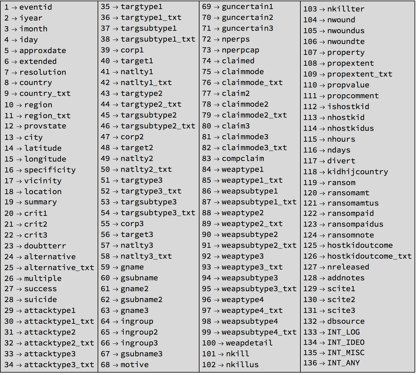
There is a "codebook" (https://www.start.umd.edu/gtd/downloads/Codebook.pdf) where the GTDB team provide more information about all of these entries. Most of the entries are quite straight forward to read. I will not go through every entry of the list now, but only use the ones I need. If in doubt, you can always consult the codebook.
Where do attacks happen?
First we visualise where terrorism incidents happen in the world. Entries 14 and 15 are the longitude and latitude of an event. Here are the first 10 events:
gtdb[[1, -11 ;; -2, {14, 15}]]

I will use a representation I have now used in several other posts. I think that it is pretty intuitive to read.
toCoordinates[coords_] := FromSphericalCoordinates[{#[[1]], Pi/2 - #[[2]], Mod[Pi + #[[3]], 2 Pi, -Pi]}] & /@ (Flatten[{1., #/360*2 Pi}] & /@ coords)
lengths[inputdata_] := 2.*(inputdata/Max[inputdata])
myGeoHistogram[data_, radius_] := Show[SphericalPlot3D[radius, {u, 0, Pi}, {v, 0, 2 Pi}, Mesh -> None, TextureCoordinateFunction -> ({#5, 1 - #4} &),
PlotStyle -> Directive[Specularity[White, 10], Texture[Import["/Users/thiel/Desktop/backgroundimage.gif"]]], Lighting -> "Neutral", Axes -> False, RotationAction -> "Clip", Boxed -> False, PlotPoints -> 100, PlotRange -> {{-3, 3}, {-3, 3}, {-3, 3}}, ImageSize -> Full],
Graphics3D[Flatten[{Green, Thick, Line[{#[[1]], (radius + #[[2]])*#[[1]]}] & /@ Transpose[{toCoordinates[#[[All, 1]]], lengths[#[[All, 2]]]} &@data]}]]]
The background image is attached to this post. With that we can represent the events like so:
myGeoHistogram[Transpose@{DeleteCases[gtdb[[1, -2071 ;; -2, {14, 15}]], {"", ""}], ConstantArray[1, Length[DeleteCases[gtdb[[1, -2071 ;; -2, {14, 15}]], {"", ""}]]]}, 3.]
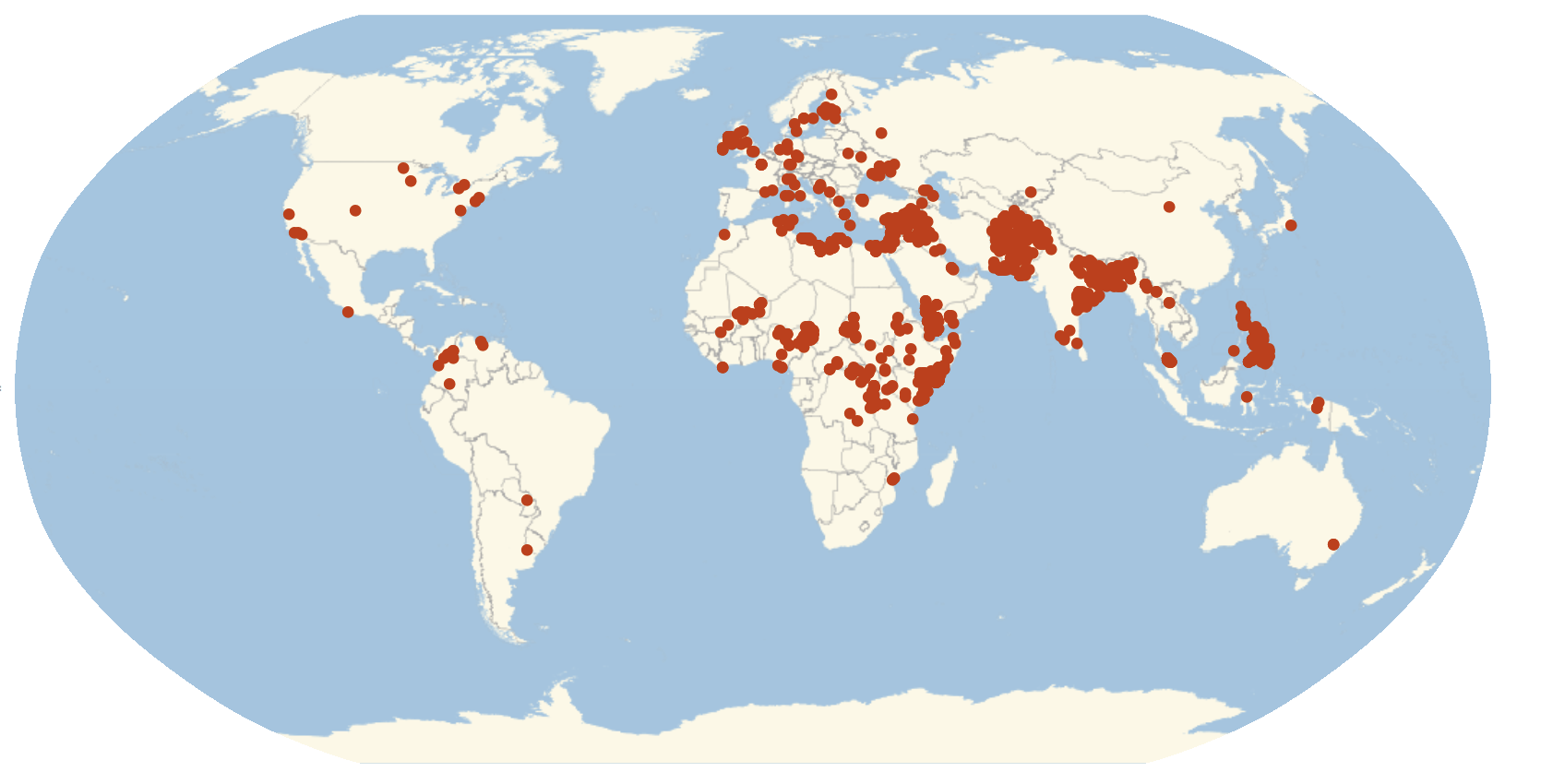
There is obviously a very high number of events in the Middle East and in Afghanistan. Here is another visualisation of the same data:
GeoListPlot[GeoPosition /@ DeleteCases[gtdb[[1, -2071 ;; -2, {14, 15}]], {"", ""}], GeoRange -> "World", GeoProjection -> "Robinson", ImageSize -> 800]
Number of people killed
In column 101 each entry contains information on the number of people that were killed in the attack. We can make a histogram of that.
ListLogLogPlot[SortBy[Select[DeleteCases[Tally[Round /@ gtdb[[1, 2 ;; -2]][[All, 101]]], {"", _}], #[[1]] >= 1 &], First], PlotTheme -> "Marketing",
 ImageSize -> Large, LabelStyle -> Directive[Bold, 16], FrameLabel -> {"number of casulties", "number of incidents"}]
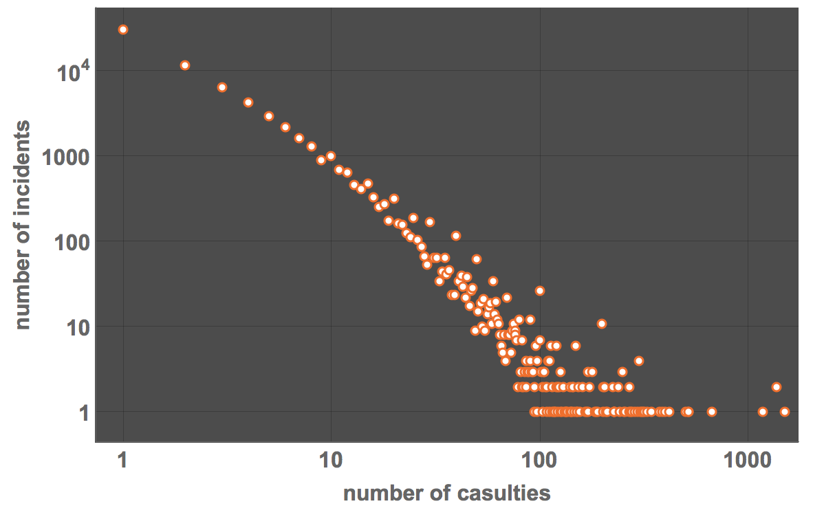
It turns out that occasionally the number of people killed is not an integer.
Select[SortBy[Select[DeleteCases[Tally[gtdb[[1, 2 ;; -2]][[All, 101]]], {"", _}], #[[1]] >= 1 &], First][[All, 1]], # - Floor[#] != 0 &]
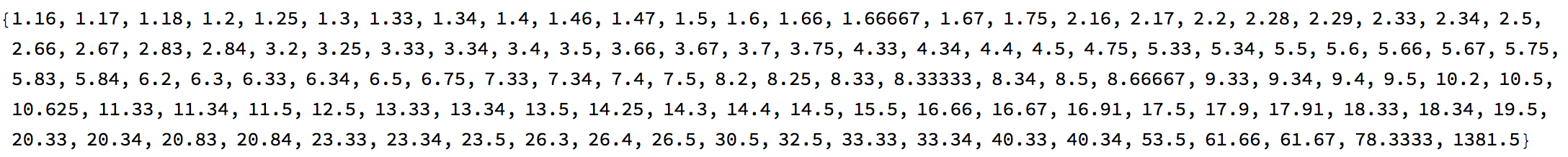
In the codebook they say:
When several cases are linked together, sources sometimes provide a cumulative fatality total for all of the events rather than fatality figures for each incident. In such cases, the preservation of statistical accuracy is achieved by distributing fatalities across the linked incidents. Depending on the number of linked events and the cumulative total of fatalities, it is possible for fractions to appear in the fatality field for individual events.
This is why I used the "Round" function of the histogram. As expected there are fewer incidents with very high casualty numbers. In fact, the behaviour seems to be nearly "scale-free", i.e. a straight line in a log-log plot.
Country by country
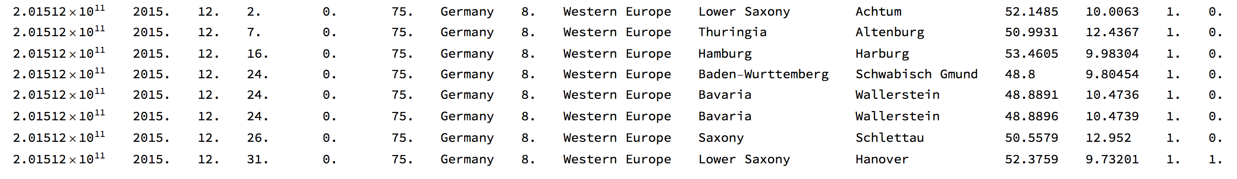
We can also look at the data for a specific country. These are incidents in Germany all from December 2015:
Select[gtdb[[1, -1071 ;; -2]], #[[9]] == "Germany" &] // TableForm
Here are descriptions of what happened:
Select[gtdb[[1, -1071 ;; -2]], #[[9]] == "Germany" &][[All, 19]] // TableForm
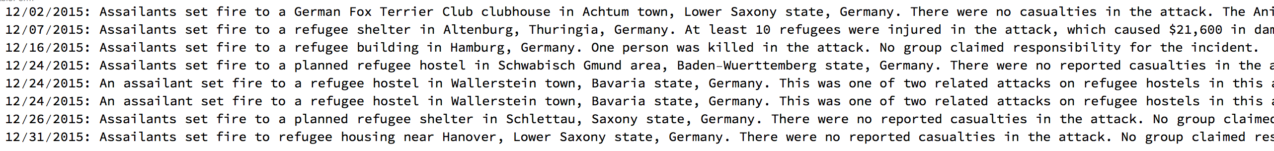
Most of the attacks are on refugee shelters.
Attacks over the years
The dataset also contains historic case since 1970. We can extract the years from the database like this:

Note that there are no incidents reported for 1993. Let's sort this by year and tally:
attacksvsyear = Transpose[{DateObject[ToString[#]] & /@ DeleteCases[Range[1970, 2015], 1993], Length /@ GatherBy[gtdb[[1, All]], #[[2]] &][[2 ;;]]}]
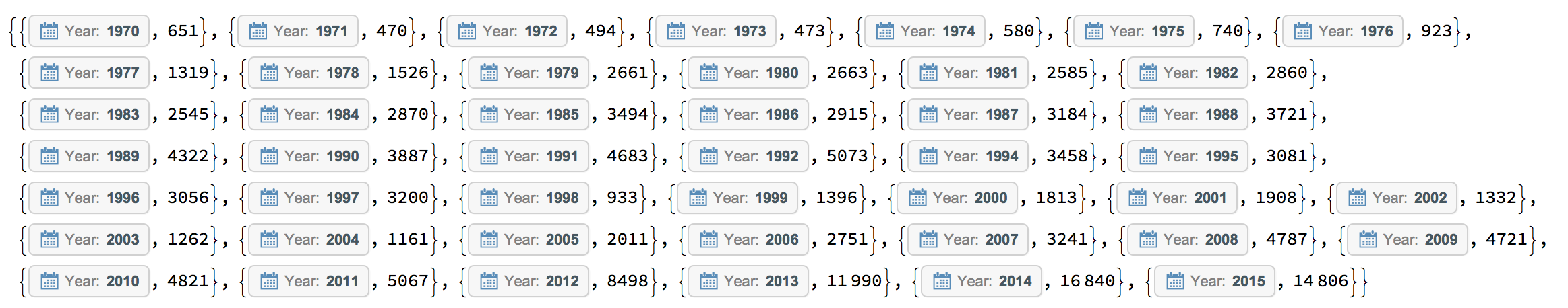
Now we can plot the number of incidents from 1970 until 2015.
DateListPlot[attacksvsyear, Background -> Black, PlotStyle -> Directive[RGBColor[{0.7, 0, 0}], Thickness[0.005]],
 LabelStyle -> Directive[Yellow, Bold, Medium, FontSize -> 22], Filling -> Bottom, FillingStyle -> RGBColor[1, 0.5, 0.5],
 ImageSize -> Full, PlotRange -> All]
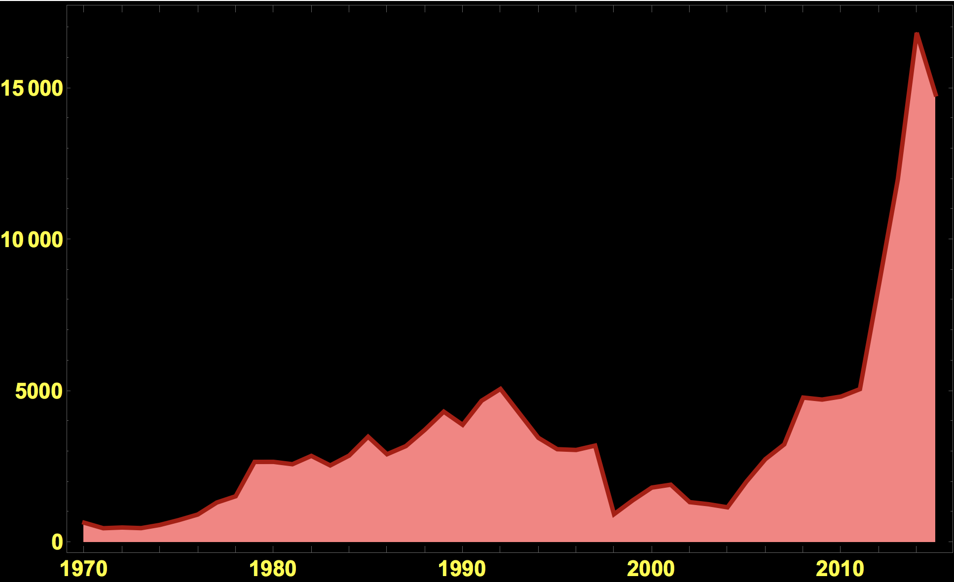
On the GTDB website they say that some time in the middle of the sequence the methodology of the data acquisition has changed, so the methodology might not be completely consistent. In particular at the end of 2011 the method has changed (see page 4 of the codebook); it has been tried though to be as consistent as possible.
Graphics of geo-distribution of attacks and casualties
The following image shows terrorism incidents on a map of the world; the sizes of the disks correspond to the number of people killed. Here are the deadly attacks of 2015:
GeoGraphics[Join[{Red}, GeoDisk[{#[[1]], #[[2]]}, Sqrt[#[[3]]]*Quantity[40, "Kilometers"]] & /@
Select[Cases[gtdb[[1, -14806 ;; -2, {14, 15, 101}]], {_Real, _Real, _Real}], #[[3]] > 0. &]], GeoRange -> "World",
GeoProjection -> "Mercator", ImageSize -> Full, GeoBackground -> "CountryBorders"]
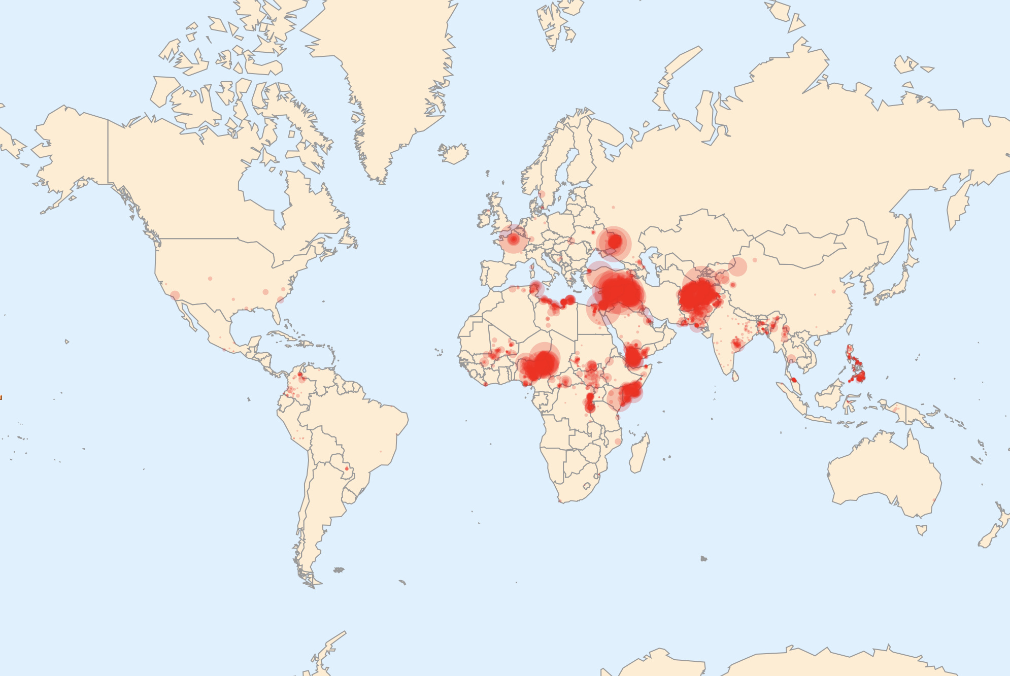
We can change the styling a little bit:
styling = {GeoBackground -> GeoStyling["StreetMapNoLabels", GeoStylingImageFunction -> (ImageAdjust@ColorNegate@ColorConvert[#1, "Grayscale"] &)], GeoScaleBar -> Placed[{"Metric", "Imperial"}, {Right, Bottom}], GeoRangePadding -> Full, ImageSize -> Large};
GeoGraphics[Join[{Red}, GeoDisk[{#[[1]], #[[2]]}, Sqrt[#[[3]]]*Quantity[40, "Kilometers"]] & /@ Select[Cases[gtdb[[1, -8000 ;; -2, {14, 15, 101}]], {_Real, _Real, _Real}], #[[3]] > 0. &]], GeoRange -> "World", GeoProjection -> "Equirectangular", ImageSize -> Full, styling]
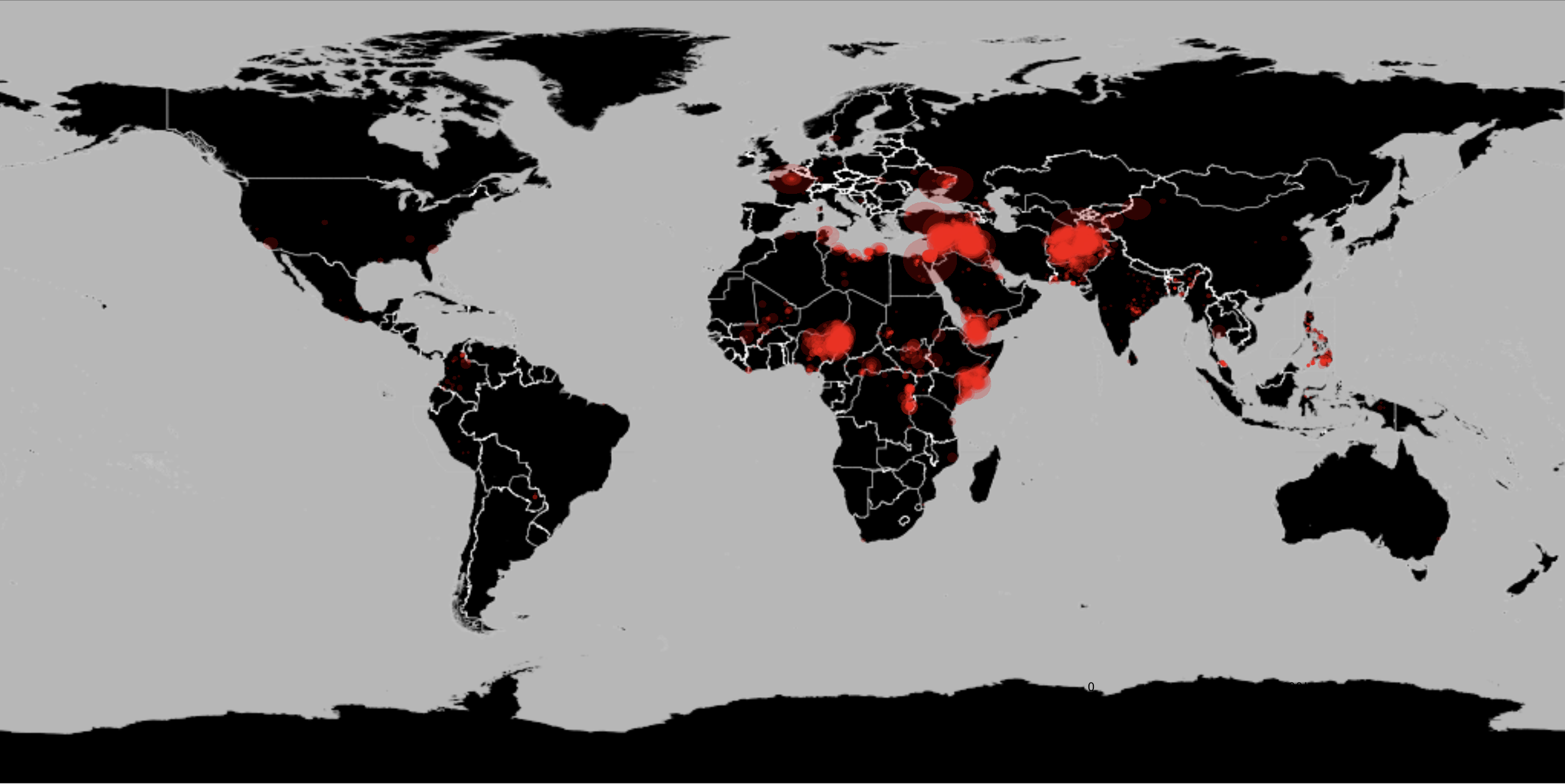
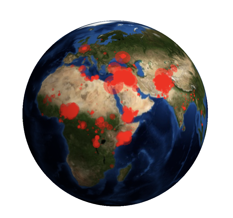
We can now also plot this on a 3D representation of the world:
backgrnd = GeoGraphics[Join[{Red, GeoStyling[Opacity[0.4]]}, GeoDisk[{#[[1]], #[[2]]}, Sqrt[#[[3]]]*Quantity[40, "Kilometers"]] & /@
Select[Cases[gtdb[[1, -8000 ;; -2, {14, 15, 101}]], {_Real, _Real, _Real}], #[[3]] > 0. &]], GeoRange -> "World", GeoBackground -> "Satellite" ,
GeoProjection -> "Equirectangular", ImageSize -> Large]; SphericalPlot3D[3, {u, 0, Pi}, {v, 0, 2 Pi},
 Mesh -> None, TextureCoordinateFunction -> ({#5, 1 - #4} &), PlotStyle -> Directive[Specularity[Black], Texture[backgrnd]],
 Lighting -> "Neutral", Axes -> False, RotationAction -> "Clip", Boxed -> False, PlotPoints -> 100, PlotRange -> {{-3, 3}, {-3, 3}, {-3, 3}}, ImageSize -> Large]
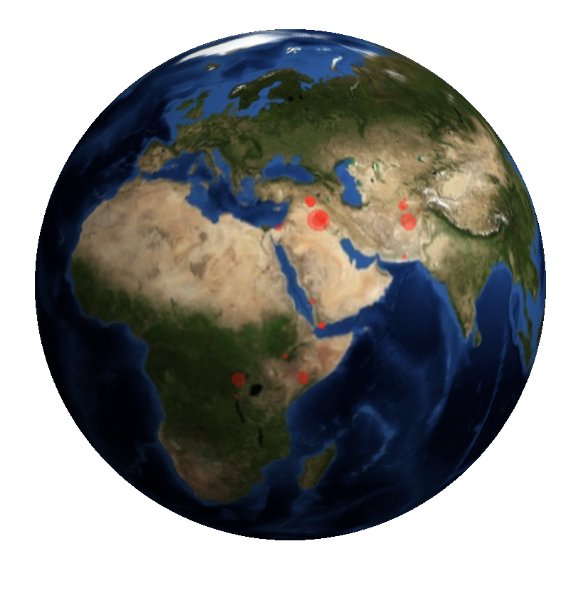
We can also build a function to deal with data of the form {lat,lon,nkilled}. First, we prepare the data:
datalonlatkill = Select[Cases[gtdb[[1, -80 ;; -2, {14, 15, 101}]], {_Real, _Real, _Real}], #[[3]] > 0. &];
then we generate the function:
myBlobPlot[data_] := Module[{}, backgrnd = GeoGraphics[
Join[{Red, GeoStyling[Opacity[0.4]]}, GeoDisk[{#[[1]], #[[2]]}, Sqrt[#[[3]]]*Quantity[40, "Kilometers"]] & /@ data],
GeoRange -> "World", GeoBackground -> "Satellite" , GeoProjection -> "Equirectangular", ImageSize -> Large];
SphericalPlot3D[3, {u, 0, Pi}, {v, 0, 2 Pi}, Mesh -> None, TextureCoordinateFunction -> ({#5, 1 - #4} &),
PlotStyle -> Directive[Specularity[Black], Texture[backgrnd]], Lighting -> "Neutral", Axes -> False, RotationAction -> "Clip",
Boxed -> False, PlotPoints -> 100, PlotRange -> {{-3, 3}, {-3, 3}, {-3, 3}}, ImageSize -> Large]]
and plot:
myBlobPlot[datalonlatkill]
Let's try to plot this as a movie in 3 month windows. First we need to create data with also contains the year and month of the attack.
datalonlatkill = Select[Cases[gtdb[[1, ;; -2, {14, 15, 101, 2, 3}]], {_Real, _Real, _Real, _, _}], #[[3]] > 0. &];
Then we calculate a list of positions in the data of the "last case belonging to one of the particular time window.
threemonthwindows = Flatten[Table[{_, _, _, i, j}, {i, 1970., 2015., 1.}, {j, {3., 6., 9., 12.}}], 1];
Then we calculate the indices of all elements in each window.
borders = Prepend[Quiet[Table[Position[datalonlatkill, Cases[datalonlatkill, threemonthwindows[[k]]][[-1]]][[1, 1]], {k, 1, Length[threemonthwindows]}] /. {}[[1, 1]] -> Missing["NotAvailable"]], 0];
and then the bins
bins = {1, 0} + # & /@ Partition[borders, 2, 1];
Now we can make the 3D globe for all time points:
myBlobPlot[datalonlatkill[[#[[1]] ;; #[[2]]]][[All, 1 ;; 3]]] &@ bins[[22]]
Now we want to create a little animation. The globe should turn and show a sequence of states. I could use something like rotate or Viewpoint, but chose to do something a bit different: I will actually move the background image and map it onto a stable sphere. First of all we need to know the dimensions of the background image
backgrnd // ImageDimensions
(*{576,288}*)
Let's remove the bins without any events and count how many there are.
Cases[bins, {_?NumberQ, _?NumberQ}] // Length
(*179*)
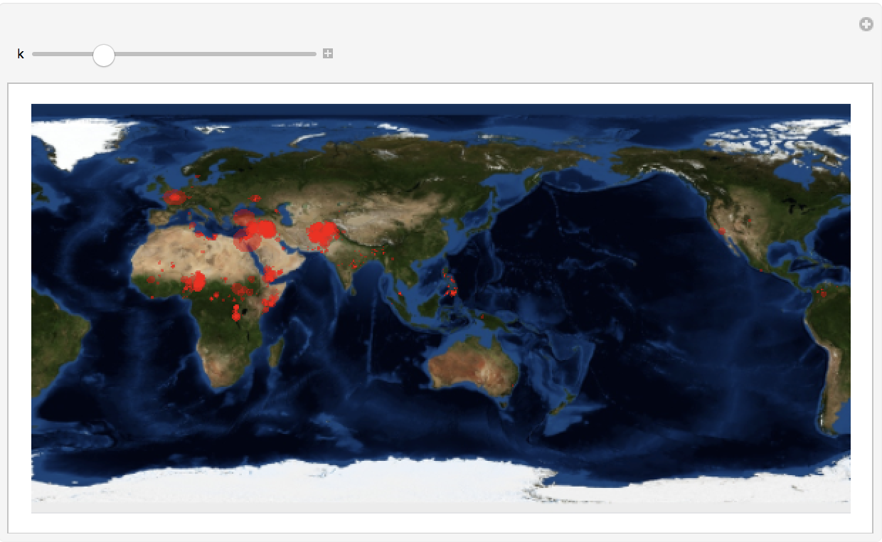
We can now make a Manipulate structure to get the idea. As I move the slider the image is cut into to pieces and reassembled. It is actually quite responsive.
Manipulate[ImageAssemble[{ImageCrop[backgrnd, {576 - k, Full}, Left], ImageCrop[backgrnd, {k, Full}, Right]}], {k, 1, 575, 1}]
Now we can use this idea to "rotate" the background and map it onto the sphere. I generate the frames that will make up my movie.
Monitor[frames =
   Table[backgrnd =
     GeoGraphics[
      Join[{Red, GeoStyling[Opacity[0.4]]},
       GeoDisk[{#[[1]], #[[2]]},
          Sqrt[#[[3]]]*
           Quantity[40,
            "Kilometers"]] & /@ (datalonlatkill[[#[[1]] ;; \
#[[2]]]][[All, 1 ;; 3]] &@ (Cases[
             bins, {_?NumberQ, _?NumberQ}][[k]]))],
      GeoRange -> "World", GeoBackground -> "Satellite" ,
      GeoProjection -> "Equirectangular", ImageSize -> Large];
    backgrnd =
     ImageAssemble[{ImageCrop[backgrnd, {576 - Mod[k*10, 576], Full},
        Left], ImageCrop[backgrnd, {Mod[k*10, 576], Full}, Right]}];
    Image[
     SphericalPlot3D[3, {u, 0, Pi}, {v, 0, 2 Pi}, Mesh -> None,
      TextureCoordinateFunction -> ({#5, 1 - #4} &),
      PlotStyle -> Directive[Specularity[Black], Texture[backgrnd]],
      Lighting -> "Neutral", Axes -> False, RotationAction -> "Clip",
      Boxed -> False, PlotPoints -> 100,
      PlotRange -> {{-3, 3}, {-3, 3}, {-3, 3}}, ImageSize -> Large,
      Background -> Black]], {k, 1, 179}];, k]
We can now animate the frames or export them.
Monitor[Do[Export["~/Desktop/GTDBmovie/frame" <> ToString[1000 + k] <> ".jpg", frames[[k]], ImageResolution -> 100], {k, 1, Length[frames], 1}],k]
The resulting video is shown at the top of this post.
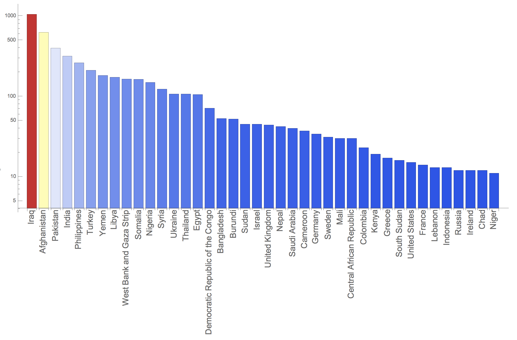
Incidents by country
The following histogram looks at the number of cases in different countries; only the first 40 are displayed.
BarChart[#[[All, 2]], ChartLabels -> (Rotate[Style[#, 16], Pi/2] & @@@
Reverse[SortBy[Tally[gtdb[[1, -5000 ;;, 9]]], Last]][[1 ;; 40]]), ColorFunction -> Function[{height}, ColorData["Temperature"][height]],
ImageSize -> Full, ScalingFunctions -> "Log"] & @ Reverse[SortBy[Tally[gtdb[[1, -5000 ;;, 9]]], Last]][[1 ;; 40]]
Other information in the database
Again, this is a very rich database and much more information can be extracted. Let's look at textual data. We can first find the positions of textual data in the entries like so:
textpos = Flatten[Position[gtdb[[1, 1]], #] & /@ Select[gtdb[[1, 1]], StringContainsQ[#, "_txt"] &]];
We can now create a lookup table for these columns.
Rule @@@ Transpose[{textpos, gtdb[[1, 1, textpos]]}]

In column 85 for example there are the weapon types.
gtdb[[1, 2 ;; 100, 85]]
Here is a tally of frequently used weapons.
Reverse@SortBy[Tally[RandomChoice[gtdb[[1, All, 85]], 5000]], Last] // TableForm
We can create a WordCloud to visualise this:
WordCloud[RandomChoice[gtdb[[1, All, 85]], 1000], ImageSize -> Large, WordOrientation -> {{0, \[Pi]/3}}]

Have the weapons changed over time? Let's look at the first 5000 attacks:
Reverse@SortBy[Tally[gtdb[[1, 2 ;; 5000, 85]]], Last] // TableForm
And the last 5000.
Reverse@SortBy[Tally[gtdb[[1, -5000 ;;, 85]]], Last] // TableForm
There seem to be more vehicle based attacks. Let's look at that more closely:
Reverse@SortBy[Tally[gtdb[[1, 2 ;;, 85]]], Last] // TableForm
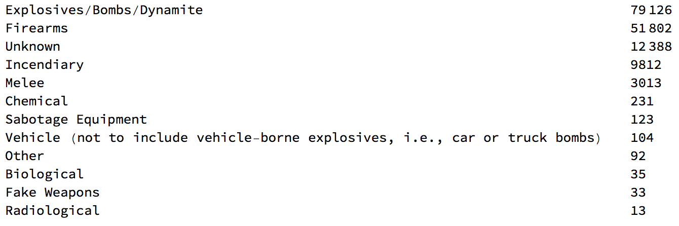
Let's define
attacktypes = Reverse@SortBy[Tally[gtdb[[1, 2 ;;, 85]]], Last][[All, 1]]

We can now look at overlapping windows of 5000 and count the weapons used.
Monitor[weaponsovertime = Table[Count[gtdb[[1, 2 + k*50 ;; 5002 + k*50, 85]], #] & /@ attacktypes, {k, 0, 3000}], k]
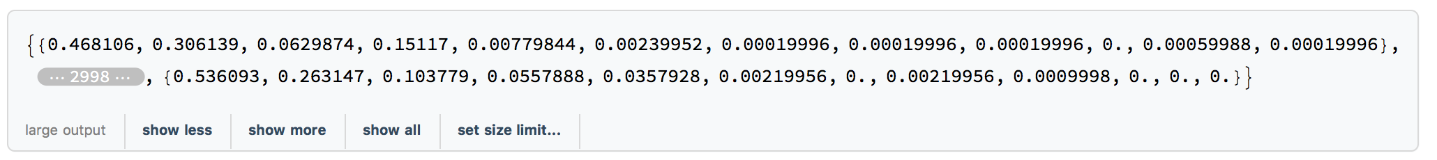
Let's try to make this nice. First we normalise.
(1. #/Total[#]) & /@ (weaponsovertime[[1 ;; 3000]])
Now we plot that:
ListLinePlot[Transpose[Accumulate /@ ((1. #/Total[#]) & /@ (Reverse /@ weaponsovertime[[1 ;; 3000]]))], PlotRange -> All,
Filling -> (#[[2]] -> {#[[1]]} & /@ Partition[Range[12], 2, 1]), ImageSize -> Large, PlotLegends -> Reverse@attacktypes, LabelStyle -> Directive[Bold, 14], AxesLabel -> {"Time / au", "percentage"}]
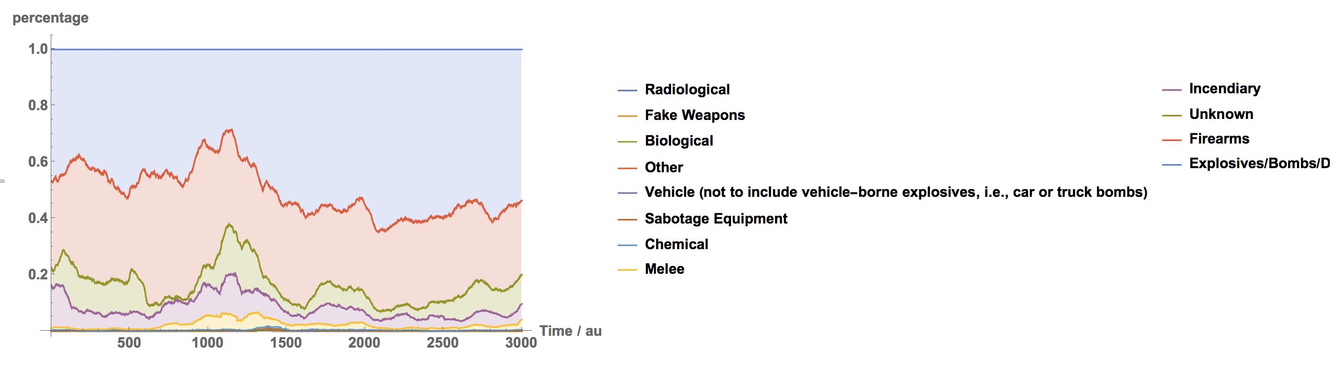
Note that the legend is in "reverse order" the top most curve in the list corresponds to the last entry in the legend.
Conclusion
This post is only scratching the surface of what is possible with this data set. I find it very exciting that with the Wolfram Language and freely available databases you can answer your own questions about many of the most urgent questions we face today.


