To put it in simple terms, if ArcCos did not evaluate to a number it would be fairly useless. Same for Log and all the rest.

As for multiple solutions to trig equations, there is Solve and Reduce. Example:

In[203]:= Solve[Cos[x] == 1, x]

(* Out[203]= {{x ->  ConditionalExpression[2 \[Pi] C[1], C[1] \[Element] Integers]}} *)

Good responses all around, and I agree. It's useful to think about the conditions where you expect an inverse function to exist, and how are the inverse functions defined or calculated from first principles?

You should conclude that the notion of an inverse function is essentially a local concept, limited to domains where the direct function is either strictly increasing or strictly decreasing.

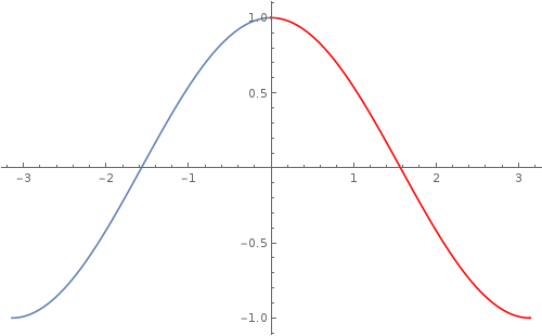
Then, if necessary, you can program functionality to "patch" your direct and inverse functions. For example:

Show[
 Plot[Cos[x], {x, -Pi, 0}],
 Plot[Cos[x], {x, 0, Pi}, PlotStyle -> Red], PlotRange -> All,
 ImageSize -> 500
 ]

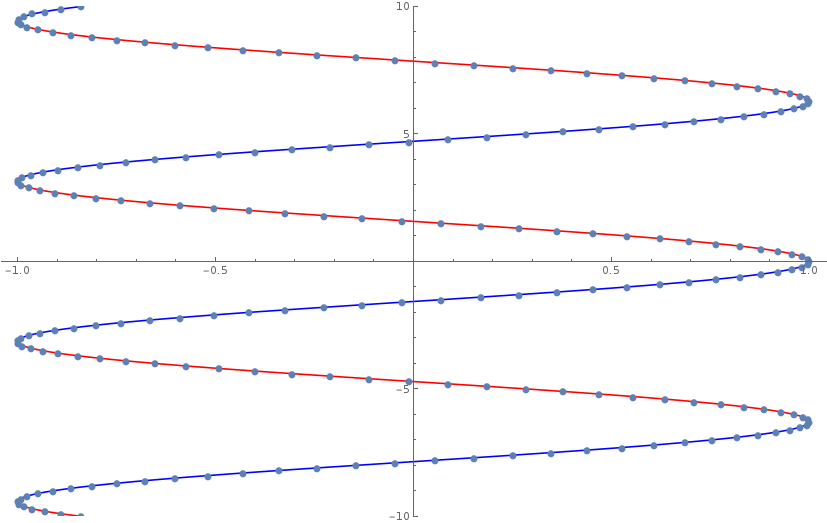
Extrapolate this patching scheme to the entire domain, taking advantage of translation ivariance. Then permute $x$ and $y$ axis, and you will calculate the following patched inverse function

Show[

Plot[
-ArcCos[x] + 2 Pi # & /@ Range[-5, 5], {x, -1, 1}, 
PlotRange -> {-10, 10}, PlotStyle -> Blue],
Plot[
ArcCos[x] + 2 Pi # & /@ Range[-5, 5], {x, -1, 1}, 
PlotRange -> {-10, 10}, PlotStyle -> Red],
ListPlot[{Cos[#], #} & /@ (Range[-150, 100]/10), 
PlotMarkers -> {Automatic, 10}]]

Thanks, Brad.

Perhaps ArcTan[x,y] instead of ArcTan[x/y]

V[r_, ?_] := Exp[-(r - 1)^2]*(Exp[-?^2] + Exp[-(? - 2 ?/3)^2] + Exp[-(? + 2 ?/3)^2]) /. ?->ArcTan[x, y];
TransformedField["Polar"->"Cartesian", V[r, ?], {r, ?}->{x, y}];
ContourPlot[%, {x, -2, 2}, {y, -2, 2}, PlotRange -> All]

Read the help page carefully to make certain the order of x,y and x/y are correct in your ArcTan.

In V10.1 it displays without the discontinuity.

In V11.1 it displays with the discontinuity.

Perhaps you can think very carefully, write your own version of TransformedField and see if you can avoid the discontinuity.

Perhaps someone can look at the internal details of TransformedField and see if the implementation has shown "unexpected behavior".

I think you should be careful with this plot, and it looks like you are headed in a wrong direction. The function you give isn't $2\pi$ periodic, as can easily be seen by explicit computation of function values

V[r_, \[CurlyPhi]_] :=   Exp[-(r - 1)^2]*(Exp[-\[CurlyPhi]^2] +  Exp[-(\[CurlyPhi] - 2 \[Pi]/3)^2] + Exp[-(\[CurlyPhi] + 2 \[Pi]/3)^2])
N@V[1, 0]
N@V[1, 2 Pi]

1.02489
2.3982*10^-8

So the function domain isn't planar. Then why would you use polar coordinates?

Maybe I'm reading too much into your symbolism, but it looks like you're trying to define a potential function with a central saddle point, and a few equally spaced minima. The best way to do this is to insert power series expansions into the elements of a $2\times2$ matrix, apply a symmetry constraint to matrix elements and polynomial variables to reduce degrees of freedom, and finally diagonalize the matrix. If you do all this right, the lower energy eigenvalue surface should be a nice potential function with all your desired extremal properties and a conical intersection at the origin. These sort of potential surfaces are used in the setting of the vibronic Jahn-Teller effect. A good-enough article is: Effects of higher order Jahn-Teller coupling on the nuclear dynamics .