Hello Jef,
( I have edited this post. My beginners attempt was pretty clumsy -- I've since learned how to do better.)
This can be done in Mathematica using Lagrangian mechanics. The code below (something I once did for fun) solves a similar problem using that method. It considers a roller coaster car on a parabolic track with a simple damping. The Lagrangian is T-V, with T = kinetic energy and V = potential energy. It uses the VariationalMethods package to obtain the equations of motion left hand side from the Lagrangian. The method of Lagrange multipliers (one is needed) is used to enforce the constraint that the car follows the track. That produces forces of constraint which appear on the right hand side of the equations of motion, together with the damping force.
For your problem, there is an additional term required in the kinetic energy Iw^2, where I is the moment of inertia (related to your R) and w is the radian velocity. Of course, the radian velocity is related to the linear velocity of the car by the no-slip condition, so that wR = v, with v the magnitude of the velocity of the car.
It's worth noticing that once you have the equations of motion in symbolic form, you see a damped harmonic oscillator, with the oscillation frequency in the x and y directions equal and in phase. So you know a great deal about the system without actually performing a numerical simulation.
You did not indicate where you are in your learning. These methods are at the level of an advanced undergrad in physics. And if your not quite there yet may not be appropriate for now. But you clearly have an interest, so I thought you might enjoy the response.
Kind regards,
David
Remove symbols and load the VariationalMethods package
Remove["Global`*"];
Needs["VariationalMethods`"];
SetOptions[Plot, PlotRange -> All];
SetDirectory[NotebookDirectory[]];
The constraints to follow the parabola will appear as factors to a Lagrange multiplier
constraint0 = y[t] - x[t]^2;
constraint = y[t] == x[t]^2;
constraintd1 = D[constraint, {t, 1}];
constraintd2 = D[constraint, {t, 2}];
aX = D[constraint0, x[t]];
aY = D[constraint0, y[t]];
Use the variational derivative to obtain the Euler-Lagrange equations. The Lagrange multiplier and the damping factor B appear on the RHS of the equations of motion.
L = m (x'[t]^2 + y'[t]^2)/2 - m g y[t];
eqX = VariationalD[L, x[t],
t] == -\[Lambda][t] aX + \[CapitalBeta] x'[t];
eqY = VariationalD[L, y[t],
t] == -\[Lambda][t] aY + \[CapitalBeta] y'[t];
Use NDSolve to solve for the trajectory and the multipliers
tmax = 50;
equations = {constraintd2, eqX, eqY};
values = {g -> 1, m -> 1, \[CapitalBeta] -> 0.2};
{x, y, \[Lambda]} = NDSolveValue[
{
equations /. values,
x[0] == -1, x'[0] == 0, y[0] == 1, y'[0] == 0
}, {x, y, \[Lambda]}, {t, 0, tmax}];
maxTime = x[[1, 1, 2]];
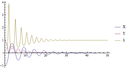
Plot x, y, and \ individualy
xy\[Lambda]Plot =
Plot[{x[t], y[t], \[Lambda][t]}, {t, 0, maxTime},
PlotLegends -> {"X", "Y",
"\[Lambda]"}]; Export["xylPlot.png", xy\[Lambda]Plot];
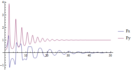
The multipler \ with its factor is the force of constraint acting on the car
fPlot = Plot[\[Lambda][t] {aX, aY} // Evaluate, {t, 0, maxTime},
PlotLegends -> {"Fx", "Fy"}]; Export["fxyPlot.png", fPlot];
Make an arrow function to plot a vector representation of the force of constraint. "a" is just a scaling factor
arrow[t_, a_] =
Arrow[{{x[t], y[t]}, {x[t], y[t]} +
a {aX \[Lambda][t], aY \[Lambda][t]}}];
Plot an animation of the equations. The arrow represents the force exerted on the car to keep it on the track
animation = Animate[
Graphics[
{
{Thick, Plot[x^2, {x, -1, 1}][[1]]},
{PointSize[0.025], Point[{x[t], x[t]^2}]},
{Red, Thick, Arrowheads[0.025], arrow[t, .12]}
}, PlotRange -> {{-1, 1}, {-.1, 1}}
], {t, 0, maxTime, .01},
DefaultDuration -> 25]