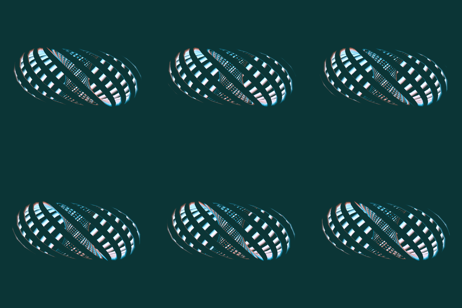
Stereo Vision
This is very similar to Rise Up, though with a $(24,23)$-torus knot rather than a $(29,-5)$-torus knot. The major difference is that, rather than stereographically projecting the knot from the 3-sphere to $\mathbb{R}^3$ and then building a tube of uniform thickness around it, I'm making the uniform tube up in the 3-sphere and projecting the whole thing down. Thanks to @Henry Segerman for the suggestion.
In order to accomplish this, I parametrized the boundary of a tubular neighborhood, found the formula for the projection, and then used ParametricPlot3D. In practice, this turned out to be quite computationally expensive. I will show the code at the end, but the code is basically incomprehensible without knowing where it came from, so I'll start with some intermediate steps.
First, we need a stereographic projection function and a function which will output a $(p,q)$-torus knot on the Clifford torus, offset by an angle $\theta$ from the standard one:
Stereo3D[{x1_, y1_, x2_, y2_}] := {x1/(1 - y2), y1/(1 - y2), x2/(1 - y2)};
pqtorus[t_, \[Theta]_, p_, q_] := ComplexExpand[Flatten[ReIm /@ (1/Sqrt[2] {E^(p I (t + \[Theta]/p)), E^(q I t)})]];
Now, the way I'm going to parametrize the boundary of a tubular neighborhood of the knot is to think of the knot as the core curve of a torus; then the second circle in the torus is the unit circle in the normal space to each point on the torus. Thinking of the knot as sitting inside $\mathbb{R}^4$, each point has a 3-dimensional normal space, namely the orthogonal complement of the tangent vector to the knot. But we only want the part of the normal space which is tangent to the sphere. Since the outward unit normal to a point $\vec{p}$ on the sphere is just $\vec{p}$ itself, this means that the normal space we want is the orthogonal complement of the plane spanned by the point itself (thought of as a vector) and the tangent vector.
So then if you run
Orthogonalize[NullSpace[{#, D[#, t]}] &[pqtorus[t, \[Theta], p, q]]]
and do a lot of simplification, you will eventually arrive at the following orthonormal basis for the normal space to pqtorus[t, \[Theta], p, q]:
pqNormal[t_, \[Theta]_, p_, q_] :=
     {{(
     Sqrt[2] (-p Cos[p t + \[Theta]] Sin[q t] +
        q Cos[q t] Sin[p t + \[Theta]]))/(
     Sqrt[3 p^2 + q^2 + (-p^2 + q^2) Cos[2 q t]] Sign[p]), -((
      Sqrt[2] (q Cos[q t] Cos[p t + \[Theta]] +
         p Sin[q t] Sin[p t + \[Theta]]))/(
      Sqrt[3 p^2 + q^2 + (-p^2 + q^2) Cos[2 q t]] Sign[p])), 0, (
     Sqrt[2] Abs[p])/Sqrt[
     3 p^2 + q^2 + (-p^2 + q^2) Cos[2 q t]]}, {(-(p^2 + q^2) Cos[
        q t] Cos[p t + \[Theta]] - 2 p q Sin[q t] Sin[p t + \[Theta]])/
     Sqrt[3 p^4 + 4 p^2 q^2 + q^4 + (-p^4 + q^4) Cos[2 q t]], (
     2 p q Cos[p t + \[Theta]] Sin[q t] - (p^2 + q^2) Cos[q t] Sin[
        p t + \[Theta]])/Sqrt[
     3 p^4 + 4 p^2 q^2 + q^4 + (-p^4 + q^4) Cos[2 q t]],
     1/2 Sqrt[(3 p^2 + q^2 + (-p^2 + q^2) Cos[2 q t])/(
      p^2 + q^2)], ((-p^2 + q^2) Sin[2 q t])/(
     2 Sqrt[3 p^4 + 4 p^2 q^2 + q^4 + (-p^4 + q^4) Cos[2 q t]])}};
Now, we get an actual parametrization for the stereographically-projected surface in 3D by running the following function:
Block[{b, p = 24, q = 23},
 b[t_, \[Theta]_] := pqNormal[t, \[Theta], p, q];
 Stereo3D[Cos[r] pqtorus[t, \[Theta], p, q] + Sin[r] (Cos[s] b[t, \[Theta]][[1]] + Sin[s] b[t, \[Theta]][[2]])]
 ]
(Of course, you can put in any integers you like for p and q).
Unfortunately, just applying ParametricPlot3D to Stereo3D[Cos[r] pqtorus[t, \[Theta], p, q] + Sin[r] (Cos[s] b[t, \[Theta]][[1]] + Sin[s] b[t, \[Theta]][[2]])] was much much slower than copy-pasting the output of the above into ParametricPlot3D, so the code below contains the entire unpleasant output of the above function.
Unfortunately, we need to set PlotPoints very high to get a remotely reasonable surface, so this is far too slow to make into a Manipulate. Here's the code I used to output the above GIF:
knot =
  With[{r = .03, viewpoint = {0, 3, 0},
    cols = RGBColor /@ {"#f54123", "#0098d8", "#0b3536"}},
   ParallelTable[
      ParametricPlot3D[
       {(-1105 Cos[r] Sqrt[4514 - 94 Cos[46 t]]
             Cos[24 t + \[Theta]] +
           2 Sin[r] (1105 Cos[
                23 t] (Sqrt[1105] Cos[24 t + \[Theta]] Sin[s] -
                 23 Sqrt[2] Cos[s] Sin[24 t + \[Theta]]) +
              24 Sin[23 t] (1105 Sqrt[2]
                   Cos[s] Cos[24 t + \[Theta]] +
                 46 Sqrt[1105]
                   Sin[s] Sin[24 t + \[Theta]])))/(-2210 Sqrt[
            2257 - 47 Cos[46 t]] + 53040 Sqrt[2] Cos[s] Sin[r] +
           1105 Cos[r] Sqrt[4514 - 94 Cos[46 t]] Sin[23 t] -
           47 Sqrt[1105]
             Sin[r] Sin[s] Sin[
             46 t]), -((1105 Sqrt[2]
               Cos[s] (-47 Cos[t + \[Theta]] +
                Cos[47 t + \[Theta]]) Sin[r] +
             2208 Sqrt[1105]
               Cos[24 t + \[Theta]] Sin[r] Sin[s] Sin[23 t] +
             1105 (Cos[r] Sqrt[4514 - 94 Cos[46 t]] -
                2 Sqrt[1105] Cos[23 t] Sin[r] Sin[s]) Sin[
               24 t + \[Theta]])/(-2210 Sqrt[2257 - 47 Cos[46 t]] +
             53040 Sqrt[2] Cos[s] Sin[r] +
             1105 Cos[r] Sqrt[4514 - 94 Cos[46 t]] Sin[23 t] -
             47 Sqrt[1105] Sin[r] Sin[s] Sin[46 t])), ((
         Cos[r] Cos[23 t])/Sqrt[2] + (
         Sqrt[2257 - 47 Cos[46 t]] Sin[r] Sin[s])/(2 Sqrt[1105]))/(
        1 - (Cos[r] Sin[23 t])/Sqrt[2] + (
         Sin[r] (-53040 Sqrt[2] Cos[s] +
            47 Sqrt[1105] Sin[s] Sin[46 t]))/(
         2210 Sqrt[2257 - 47 Cos[46 t]]))},
       {t, 0, 2 \[Theta]}, {s, 0, 2 \[Theta]}, PlotPoints -> 1000,
       PlotRange -> 2.7, ViewPoint -> viewpoint, PlotStyle -> White,
       Axes -> None, Mesh -> None, ViewAngle -> \[Theta]/9,
       ViewVertical -> {0, 0, -1}, Boxed -> False,
       Background -> cols[[-1]], ImageSize -> 540,
       Lighting -> {{"Point", cols[[1]], {3/4, 0, 0}},
          {"Point", cols[[2]], {-3/4, 0, 0}}, {"Ambient", cols[[-1]], viewpoint}}],
      {\[Theta], 0., -2 \[Theta]/23 - #, #}] &[-\[Theta]/230]
   ];

Export[NotebookDirectory[] <> "knot.gif", knot, "DisplayDurations" -> 1/50, "AnimationRepetitions" -> Infinity]