Hyperspherical Package
I've developed a package that is roughly a translation into the Wolfram Language of Chapter 6 of Classical Orthogonal Polynomials of a Discrete Variable by Arnold F. Nikiforov, Sergei K. Suslov, Vasilii B. Uvarov, titled "Hyperspherical Harmonics". The package can be downloaded from my GitHub.
As this is version 1.0 of the package, there is still much to add that is not yet included. Some notable things that are missing include the unitary transformation coefficients (aka timber coefficients) and having the coordinates work in function such as CoordinateTransformData.
Background
Hyperspherical coordinates are the higher d-dimensional analog of polar (2-d) and spherical (3-d) coordinates systems. The coordinate systems consist of one length, the hyper radius R, and d-1 hyper angles. Conceptually the coordinate transformation from hyperspherical to Cartesian in d > 3 dimensions can be built up from the smaller systems:
y2 = R Sin[a];
x2 = R Cos[a];

y3 = R Sin[b] Sin[a];
x3 = R Sin[b] Cos[a];
z3 = R Cos[b];
Based on the above pattern you might guess that the next such form is
y4 = R Sin[c] Sin[b] Sin[a];
x4 = R Sin[c] Sin[b] Cos[a];
z4 = R Sin[c] Cos[b];
w4 = R Cos[c];
and you would be correct. Each additional degree of freedom adds a new angle where the existing coordinates get a factor of sine and the new degree of freedom is R times the cosine. These are known as the canonical hyperspherical coordinates.
You can visualize the construction of coordinates using a binary tree:

The construction of coordinates then follows the rules:
- Start at the root of the tree and include the hyperradius R.
- As you move left (right) through a branching vertex, add a factor of the Sin (Cos) of the angle
- Continue until you reach a leaf.
The Wolfram Language already has the canonical hyperspherical coordinates, but they are somewhat hidden. For example, they exist in CoordinateChartData:
CoordinateChartData[{"Hyperspherical", "Euclidean", 4}, "Metric"]
(* {{1, 0, 0}, {0, #1[[1]]^2, 0}, {0, 0, Sin[#1[[2]]]^2 #1[[1]]^2}} *)
Strangely they can be found in ToPolarCoordinates and FromPolarCoordinates:
ToPolarCoordinates[{x, y, z, w}]
(* {Sqrt[w^2 + x^2 + y^2 + z^2], ArcCos[x/Sqrt[w^2 + x^2 + y^2 + z^2]], ArcCos[y/Sqrt[w^2 + y^2 + z^2]], ArcTan[z, w]}*)

FromPolarCoordinates[{R, c, b, a}]
(* {R Cos[c], R Cos[b] Sin[c], R Cos[a] Sin[b] Sin[c], R Sin[a] Sin[b] Sin[c]} *)
Regardless, the canonical structure is just one of many possible orthogonal coordinate systems with a single length and d-1 angles. The rest are considered non-canonical hyperspherical coordinates.
Tutorial
The functions defined in the Hyperspherical` context provide support for hyperspherical tree graphs in order to define non-canonical hyperspherical coordinate systems. These naturally lead to the hyperspherical harmonic functions.
This loads the package:
<< Hyperspherical`
Hyperspherical Tree Graphs
The hyperspherical tree graph is a binary tree graph with d leaves (degrees of freedom), but the order of the branches matters. The graph is directed from the root to the leaves. These graphs are a representation of the decomposition of a space into the direct sum of orthogonal subspaces.
HypersphericalTreeGraph[d]   (* create a canonical hyperspherical tree graph with d leaves *)
HypersphericalTreeGraph[{b1, b2, ...}]  (* use branching vertex syntax to create hyperspherical tree graphs *)
To indicate left versus right, a branching edge b is a rule that goes to a list of two elements. The first element indicates left and the second element indicates right. If a graph is used, then it appears as a head with a single argument that acts as a unique label. 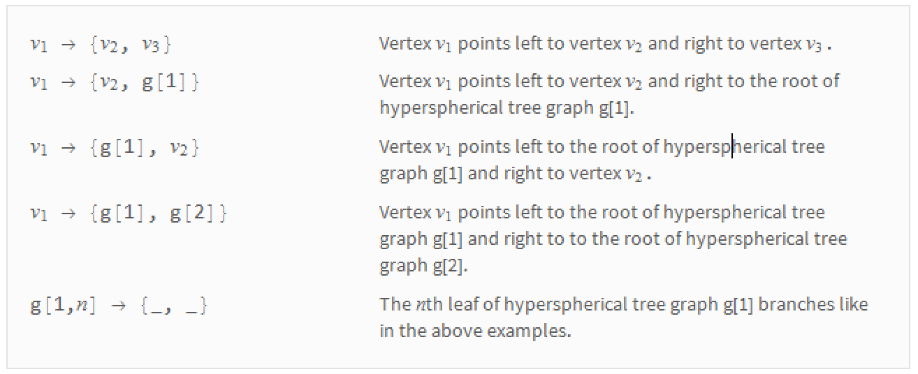
There are many ways to make a hyperspherical tree graph. For example, the following two notations have the same effect.
HypersphericalTreeGraph[{1 -> {2, 3}, 2 -> {4, 5}, 3 -> {6, 7}, 6 -> {8, 9}}];

g2 = HypersphericalTreeGraph[2];
g5 = HypersphericalTreeGraph[{1 -> {g2[A], g3[A]}}];
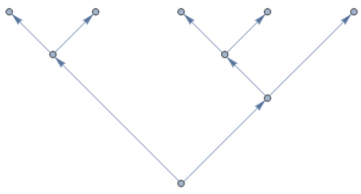
There are special branching rules as well that replace one vertex with the root of a new tree: 
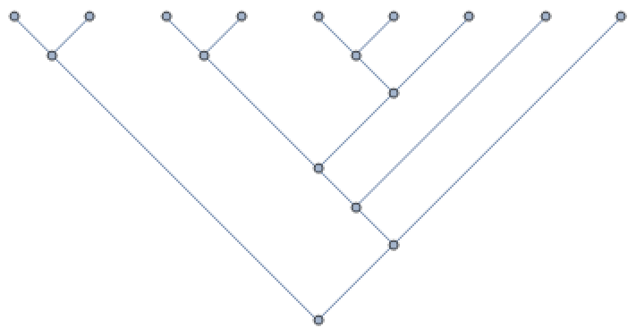
Complicated trees can then be built up quickly from earlier shapes. As more branches occur, it is easier to visualize using only lines as the edges:
HypersphericalTreeGraph[{g5[A, 3] -> g5[B]}, EdgeShapeFunction -> "Line"]
Enumerating All Graphs for Fixed Dimensionality
One interesting thing you can do with the graphs is count how many unique types can be constructed. There is a function to aid in comparing tree structures.
HypersphericalTreeSameQ[g1,g2] (* returns True if two hyperspherical tree graphs are identical *)
Using this function we can recursively add two branches to every leaf and then eliminate duplicates.
d=3
A3 = HypersphericalTreeGraph[{g2[1, #] -> g2[2]}, EdgeShapeFunction -> "Line", ImageSize -> Tiny] & /@ Range[2]

d=4
A4 = DeleteDuplicates[Join @@ Table[HypersphericalTreeGraph[{i[1, #] -> g2[2]}, EdgeShapeFunction -> "Line", ImageSize -> Tiny] &
    /@ Range[3], {i, A3}], HypersphericalTreeSameQ]

d=5
A5 = DeleteDuplicates[Flatten[Table[HypersphericalTreeGraph[{i[1, #] -> g2[2]}, EdgeShapeFunction -> "Line", ImageSize -> Tiny] &
    /@ Range[4], {i, A4}], 1], HypersphericalTreeSameQ]

d=6
A6 = DeleteDuplicates[Flatten[Table[HypersphericalTreeGraph[{i[1, #] -> g2[2]}, EdgeShapeFunction -> "Line", ImageSize -> Tiny] &
    /@ Range[5], {i, A5}], 1], HypersphericalTreeSameQ]
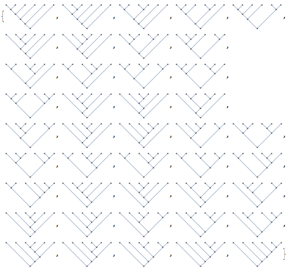
Counting the number of trees we find the famous Catalan numbers.
Length /@ {A3, A4, A5, A6} == CatalanNumber /@ Range[2, 5] (* True *)
Coordinate System Properties
Hyperspherical tree graphs are incorporated into CoordinateChartData to allow quick access to the underlying coordinate system properties.
CoordinateChartData[{"Hyperspherical","Euclidean",g},"Properties"]
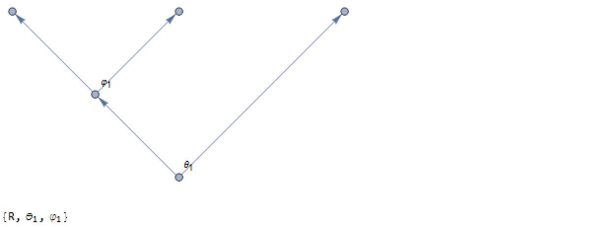
Properties like the standard coordinate names are used when using VertexLabels -> "Angles".
Standard Coordinate Names
g3 = HypersphericalTreeGraph[3, VertexLabels -> "Angles"]
CoordinateChartData[{"Hyperspherical", "Euclidean", g3}, "StandardCoordinateNames"]
Coordinate Ranges
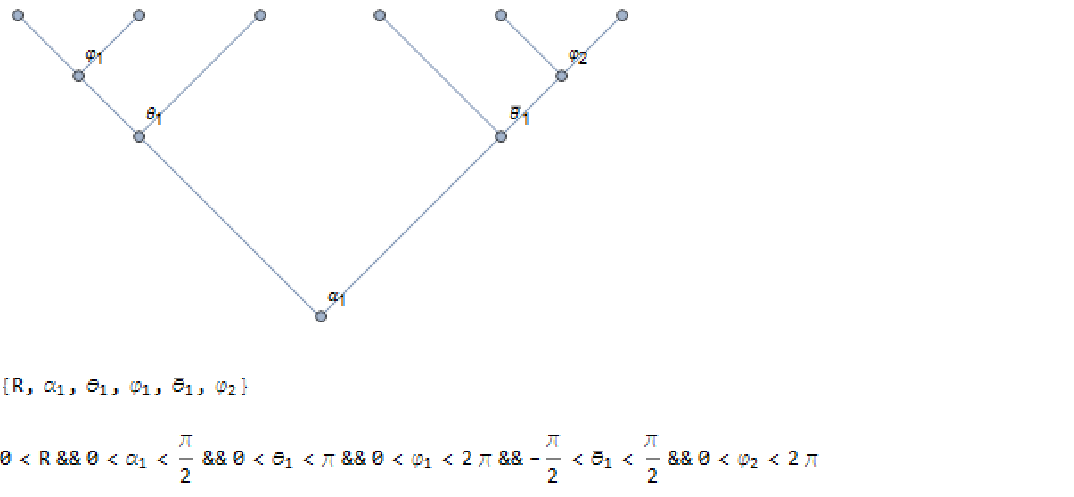
The variables have particular ranges depending on the branch structure. Note the difference between theta and theta-bar.
g3a = HypersphericalTreeGraph[{g2[A, 2] -> g2[B]}];
g6 = HypersphericalTreeGraph[{g2[A] -> {g3[A], g3a[A]}}, EdgeShapeFunction -> "Line", VertexLabels -> "Angles"]
g6coords = CoordinateChartData[{"Hyperspherical", "Euclidean", g6}, "StandardCoordinateNames"]
CoordinateChartData[{"Hyperspherical", "Euclidean", g6}, "CoordinateRangeAssumptions", g6coords]
Volume Element
The volume element is needed to compute integrals over the unit hypersphere. Using the g6 example above:
CoordinateChartData[{"Hyperspherical", "Euclidean", g6}, "VolumeFactor", g6coords]
(* R^5 Cos[Alpha1]^2 Cos[ThetaBar] Sin[Alpha1]^2 Sin[Theta1] *)
Multivariable Calculus
Functions like Grad, Div, Curl, and Laplacian also accept hyperspherical tree graphs to define hyperspherical coordinate systems.
Grad
g4 = HypersphericalTreeGraph[{g2[A] -> {g2[B], g2[C]}}];
var4 = CoordinateChartData[{"Hyperspherical", "Euclidean", g4}, "StandardCoordinateNames"] /. x_String :> ToExpression[x];
Grad[f @@ var4, var4, {"Hyperspherical", "Euclidean", g4}];
Div
Div[{f1 @@ var4, f2 @@ var4, f3 @@ var4, f4 @@ var4}, var4, {"Hyperspherical", "Euclidean", g4}]
Curl
Curl[{f1 @@ var4, f2 @@ var4, f3 @@ var4, f4 @@ var4}, var4, {"Hyperspherical", "Euclidean", g4}]
Laplacian
Laplacian[f @@ var4, var4, {"Hyperspherical", "Euclidean", g4}]
Hyperspherical Harmonics
As the SphericalHarmonicY functions are the eigenfunctions of the three-dimensional Laplacian operator in spherical coordinates, so is the HypersphericalHarmonicY functions in higher dimensions.
d=2, canonical
HypersphericalHarmonicY[{m}, {\[Phi]}, g2] (* E^(I m \[Phi])/Sqrt[2 \[Pi]] *)
d=3, canonical
In spherical coordinates, HypersphericalHarmonicY reduces to the SphericalHarmonicY function within a factor of -1.
SphericalHarmonicY[4, -1, a, b] / HypersphericalHarmonicY[{4, -1}, {a, b}, g3] // Simplify (* 1 *)
d=3, non-canonical
The inverted 3-D system resembles the standard 3-D system, but with a shift of coordinates.
SphericalHarmonicY[4, -1, \[Pi]/2 - a, b] / HypersphericalHarmonicY[{4, -1}, {a, b, g3a] // FullSimplify (* 1 *)
Angular Momenta Restrictions
The momenta can take on integer values. The hierarchy of angular momentum addition puts constraints on their values. The symbolic evaluation shows these constraints in the conditional statements.
g5 = HypersphericalTreeGraph[{1 -> {g2[A], g3[A]}}];
HypersphericalHarmonicY[{v1, v2, v3, v4}, {a1, a2, a3, a4}, g5][[2]]
(* v4 \[Element] Integers && (v1 | v2 | v3) \[Element] Integers && (-1)^v1 == (-1)^(v3 + Abs[v2]) && v1 >= v3 + Abs[v2] && v3 >= Abs[v4] *)
If the constraints are violated, then the function returns 0. For example, this fails the constraint 5 >= 2 + |-4|.
HypersphericalHarmonicY[{5, -4, 2, -1}, {a1, a2, a3, a4}, g5]
This fails the constraint (-1)^5==(-1)^(-3+1):
HypersphericalHarmonicY[{5, -3, 1, -1}, {a1, a2, a3, a4}, g5]
Eigenvalues
The eigenvalues are given by [Lambda]([Lambda]+d-2) where [Lambda] is the first angular momentum value in the list of angular momenta. This is known as the grand angular momentum.
state = HypersphericalHarmonicY[{5, -4, 1, -1}, {a1, a2, a3, a4}, g5];
Laplacian[state, {R, a1, a2, a3, a4}, {"Hyperspherical", "Euclidean", g5}] / state == (-5 (5 + 5 - 2)) / R^2 // Simplify  (* True *)
The Number of Hyperspherical Harmonics for a Fixed Grand Angular Momentum and Dimension
There is a known formula for the number of states at a fixed grand angular momentum [Lambda].
degen[\[Lambda]_, d_] := ((2 \[Lambda] + d - 2) Gamma[\[Lambda] + d - 2]) / (Gamma[\[Lambda] + 1] Gamma[d - 1])
The spherical harmonics have a degeneracy of 2L+1, where L is the grand angular momentum in three dimensions.
degen[L, 3] (* 2L + 1 *)
The number of states at a fixed [Lambda] is independent of coordinate system, as it should be. Here is a brute force enumeration for [Lambda]=3, d=4 and symmetric tree structure
case1 = Cases[Flatten[
    Table[{
        {3, L2, L3},
        HypersphericalHarmonicY[{3, L2, L3}, {a, b, c}, g4]
        },
        {L2, -3, 3, 1}, {L3, -3, 3, 1}
    ], 1], {_, Except[0]}][[All, 1]]
    (* {{3, -3, 0}, {3, -2, -1}, {3, -2, 1}, {3, -1, -2}, {3, -1, 0}, {3, -1, 2}, {3, 0, -3}, {3, 0, -1},
    {3, 0, 1}, {3, 0, 3}, {3, 1, -2}, {3, 1, 0}, {3, 1, 2}, {3, 2, -1}, {3, 2, 1}, {3, 3, 0}} *)
Here's the analogous enumeration for the canonical tree:
case2 = Cases[Flatten[
        Table[{
            {3, L2, L3},
            HypersphericalHarmonicY[{3, L2, L3}, {a, b, c}, HyperspherialTreeGraph[4]]
            },
            {L2, -3, 3, 1}, {L3, -3, 3, 1}
        ], 1], {_, Except[0]}][[All, 1]]
        (* {{3, 0, 0}, {3, 1, -1}, {3, 1, 0}, {3, 1, 1}, {3, 2, -2}, {3, 2, -1}, {3, 2, 0}, {3, 2, 1},
        {3, 2, 2}, {3, 3, -3}, {3, 3, -2}, {3, 3, -1}, {3, 3, 0}, {3, 3, 1}, {3, 3, 2}, {3, 3, 3}} *)
Note that the lists of angular momenta are different, but there lengths are the same:
Length[case1] == Length[case2] == degen[3,4] (* True *)
Orthogonality
Each state is orthonormal when integrated with respect to the unit hypersphere. For example, looking at states {3,0,0} and {3,1,-1} from the last example.
g4c = HypersphericalTreeGraph[4];
vars = CoordinateChartData[{"Hyperspherical", "Euclidean", g4c}, "StandardCoordinateNames"] /. x_String :> ToExpression[x];
vol = CoordinateChartData[{"Hyperspherical", "Euclidean", g4c}, "VolumeFactor", vars] /. R -> 1;
ranges = Sequence @@ Rest[CoordinateChartData[{"Hyperspherical", "Euclidean", g4c}, "CoordinateRangeAssumptions", vars] /. Less[a_, b_, c_] :> {b, a, c}];
state1 = HypersphericalHarmonicY[{3, 0, 0}, Rest[vars], g4c];
state2 = HypersphericalHarmonicY[{3, 1, -1}, Rest[vars], g4c];
Checking the normalization of state1:
Integrate[(state1 /. x_Complex :> Conjugate[x])*state1*vol, ranges] (* 1 *)
Checking the orthogonality of state1 and state2:
Integrate[(state1 /. x_Complex :> Conjugate[x])*state2*vol, ranges] (* 0 *)