Extracting from the Zip Archive

The data comes in a zip archive that contains three files. One file contains data on 1 million flights that took place in 2015 within the United States. It's a sample from a Kaggle dataset with over 5 million flights. I randomly sampled that data to keep the memory footprint manageable. (For now, Mathematica does not cope well with data larger than computer memory). Let's see what's in the ZIP archive. I first import and clean the data.

zipArchive = "C:\\Users\\Seth\\Downloads\\flight-delays\\flights15.zip"; 
(* you will need to use your own file name here *)

We see there are four files. The file containing the actual data is flightsOneMillion.csv.

filesInArchive = Import[zipArchive]

{"flightsOneMillion.csv", "LAirport.csv", "LAirport_ID.csv", "IATA_AirlineCodes.csv"}

Let' s import it. This will take probably 1 - 5 minutes depending on the speed of you system. Be patient! You should end up with a data structure whose dimensions are 1,000,001 x 31 (the extra row is the header).

Dimensions[csv = Import[zipArchive, filesInArchive[[1]]]]

{1000001, 31}

While we' re at it, let' s import the second and third files. We first import a file mapping conventional IATA airport codes to actual airport names. We then import a file mapping alternative airport codes to the same set of actual airport names.

Dimensions[iataCSV = Import[zipArchive, filesInArchive[[2]]]]

{6430, 2}

Dimensions[alternativeCSV = Import[zipArchive, filesInArchive[[3]]]]

{6415, 2}

Finally, we want to import a file mapping airline code abbreviations (like UA) to the actual name of the airline (United Airlines). The fourth file contains this mapping.

Dimensions[airlineCSV = Import[zipArchive, filesInArchive[[4]]]]

{15, 2}

Import the Data and Create a Dataset

Now let' s use one of the programming idioms we have developed to convert the flights CSV data into a Wolfram Language Dataset. One this is done we are going to free up some memory by using Remove on the original csv data.

flights = Dataset[Map[AssociationThread[First@csv, #] &, Rest@csv]];
Remove[csv]

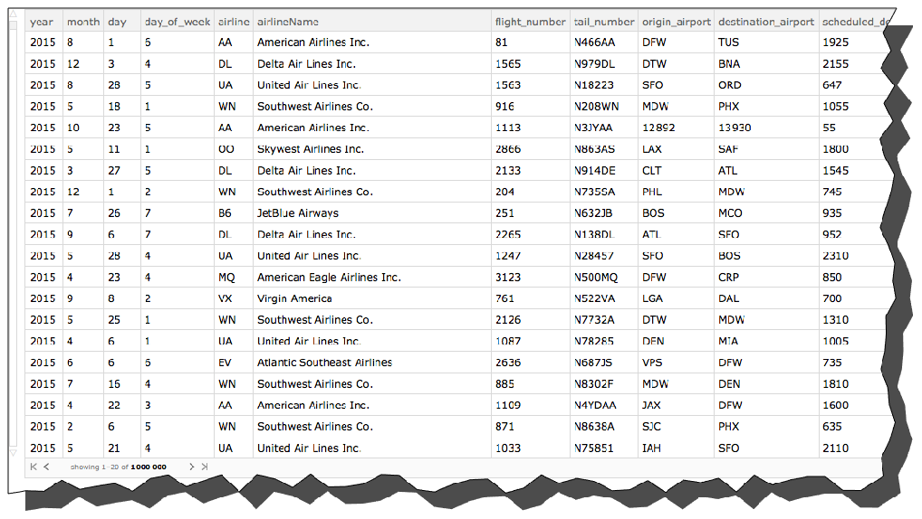
Let' s look at the first 10 rows.

flights[1 ;; 10]

Clean the Data

Changing the column headers to lower case

Notice that all the column headers are in upper case. This is a nuisance. Let's change the headers to all be lower case. To do this, remember that each row of a Dataset that has column headers is an Association. So, we use the KeyMap function, which operates on the keys of an Association instead of the values. Again, here and elsewhere, have some patience. This is pretty big data. I just printout the first four rows to make sure I have succeeded.

flights = flights[All, KeyMap[ToLowerCase]];
flights[1 ;; 4]

Add the airline name

Working with airline codes is inconvenient. So, I want to add the actual name of the airline to each row of the Dataset. To do this, I convert the mapping between airline code and airline name into an Association.

airlineCodeAssociation = Association[Apply[Rule, Rest@airlineCSV, {1}]]

And now let' s use that Association to add the airline name right after the airline. We'll add an "airlineName" column right after the "airline" column and before the "flight_number" column. To do this, we will use Insert, which lets you insert a key-value pair at a designated position in an association.

newpos = 1 + Position[Keys[flights[[1]]], "airline"][[1, 1]]

6

flights = Query[All,  Insert[#, "airlineName" -> airlineCodeAssociation[#airline], newpos] &][flights]

Working with Dates and Times

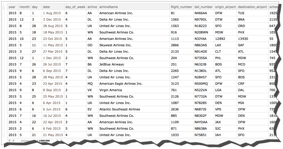
The csv file we extracted from the zip archive did not store dates and times in a particularly sensible way. We want to convert at least some of these dates and times so that they have desirable properties. I first create a function getTimeObjectFromField. The function takes an association that has some field in which time is stored as an integer like this 1455. It converts into a TimeObject representing 2:55 pm.

getTimeObjectFromField[a_Association, field_] :=  TimeObject[{Quotient[a[field], 100], Mod[a[field], 100], 0}]

Now I create three little functions that create new columns, "date," "scheduleddeparturetime" and "scheduledarrivaltime" that behave as proper dates and times in the Wolfram Language. Again I use Insert to place the new key-value pairs in the appropriate spot. I would have preferred to do this all with a single Insert rather than a chaining of multiple Insert operations, but this is currently not permitted in the Wolfram Language.

converter1 = (Insert[#, "date" -> DateObject[{#year, #month, #day}], 
     Key["day_of_week"]]) &;
converter2 = (Insert[#, 
     "scheduled_departure_time" -> 
      getTimeObjectFromField[#, "scheduled_departure"], 
     Key["departure_time"]] &);
converter3 = (Insert[#, 
     "scheduled_arrival_time" -> 
      getTimeObjectFromField[#, "arrival_time"], 
     Key["scheduled_arrival"]] &);

I'll now right compose those conversions and modify the flights Dataset.

flights = Query[All, converter1 /* converter2 /* converter3][flights]

The horrible October problem

Let' s look at the distribution of flights by origin airport by month. We'll sort the months and we'll sort the origin airports within each month according to the number of flights that originated from there. The sort is most flights to least flights.

flightsByMonthAndOrigin = 
 Query[GroupBy[#month &] /* KeySort, 
   GroupBy[#"origin_airport" &] /* ReverseSort, Length][flights]

What you can see is that ATL and ORD come out on top except during month 10 (October) when the mysterious airports 10397 and 13930 have the most fights. Those airport codes do not have the typical 3 letters of IATA codes. In fact, what appears to have happened is that a different coding system was used during October.

If we are to do proper analysis, we need for our airport codes to be consistent. We have two files that we've already imported that are going to help us straighten things out. We have iataCSV, which shows the relationship between IATA code and actual airport name, and we have alternativeCSV, which shows the relationship between alternative airport code and actual airport name. Since the two files appear to have a common piece of data -- actual airport name -- we should be able to use a JoinAcross operation to create a mapping between alternative airport code and IATA code. Once we have this mapping we can clean up the data.

Let' s start by creating two lists of Associations.

iataAssociation = Map[AssociationThread[{"IATA_Code", "airportName"}, #] &,  Rest@iataCSV]

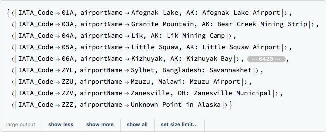
alternativeAssociation = Map[AssociationThread[{"alternative_Code", "airportName"}, #] &, Rest@alternativeCSV]

We can now use a JoinAcross operation to link up the two Associations.

airportCodesAssociation =  JoinAcross[iataAssociation, alternativeAssociation, "airportName"]

We now just create a simple association that goes from alternative code to IATA code.

airportCodeTranslator =  Query[Association, Slot["alternative_Code"] -> Slot["IATA_Code"] &][airportCodesAssociation]

We now write a function that takes an argument s. If s is a key in airportCodeTranslator, the function outputs the value for that key (an IATA code). If not, the function outputs s (the original code).

airportTranslate[s_] := Lookup[airportCodeTranslator, s, s]

We can now fix the October problem.

flights = 
 Query[All, 
   Association[#, 
     "origin_airport" -> airportTranslate[#"origin_airport"], 
     "destination_airport" -> 
      airportTranslate[#"destination_airport"]] &][flights]

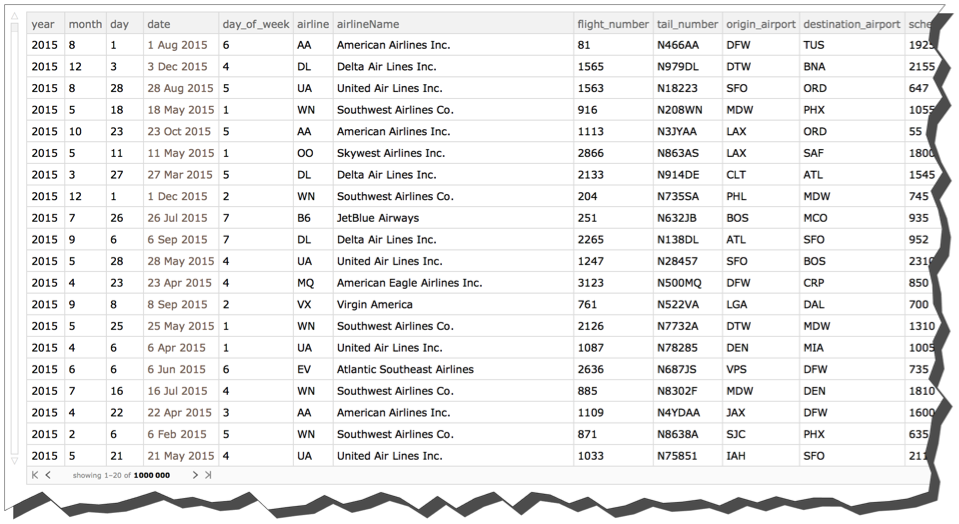
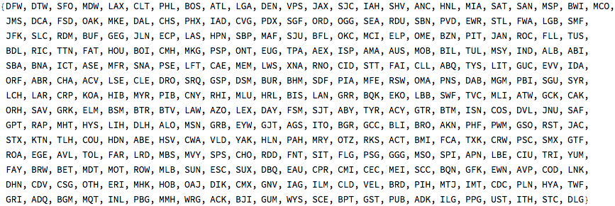
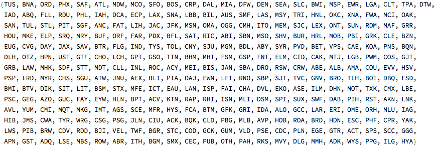
Let' s rerun our code that examines airports by months and see if the problem is gone. All the origin and destination airports now have three letter codes. The October problem appears to be fixed!

Normal@flights[DeleteDuplicates, #"origin_airport" &]

Normal@flights[DeleteDuplicates, #"destination_airport" &]

Getting rid of flights for which we have no arrival delay information

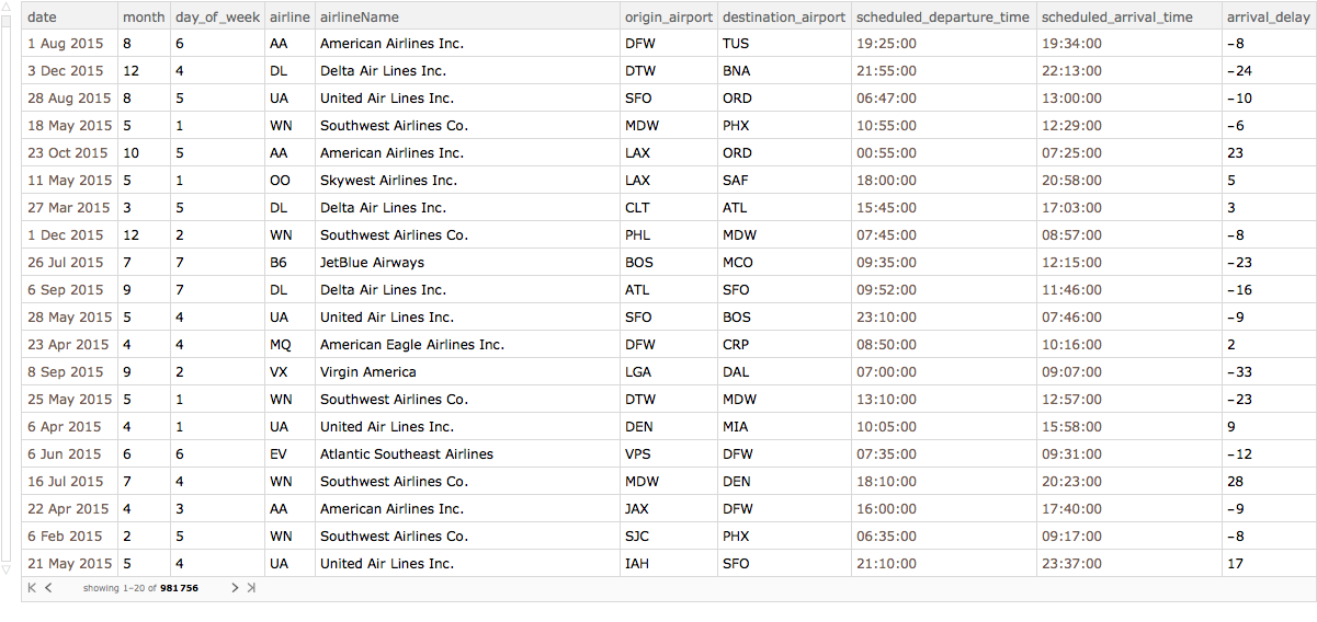
We have one last piece of clean up to do. Most of our analysis from here on in is going to deal with arrival delays. Rather than rewrite every piece of code to Select only those flights for which we have such information, let's create a new Dataset that filters out flights missing this critical information. Moreover, there are only some of the columns that we are going to deal with. For example, I really don't care about the tail number of the flight. So we can reduce the memory footprint of the Dataset. We will call the new dataset by the short name ds.

wantedColumns = {"date", "month", "day_of_week", "airline", 
   "airlineName", "origin_airport", "destination_airport", 
   "scheduled_departure_time", "scheduled_arrival_time", 
   "arrival_delay"};
ds = Query[Select[NumericQ[#"arrival_delay"] &], wantedColumns][flights]

Analysis

Late Arrivals and Creation the fractionLateAssociation function

Let' s write a fairly complex function that takes a list of potential delay thresholds and determines the fraction of flights that are above each of those values. We'll know for example what fraction of flights have arrival delays of more than 5 minutes and 15 minutes and 60 minutes. We're going to do this using something called an EmpiricalDistribution and a SurvivalFunction. We have not seen these yet, but just accept that they work.

Let' s create a list of delay thresholds about which we might care.

delays = {0, 5, 10, 15, 30, 60, 120}

Here' s our function. It is called lateness. There are two optional arguments. The keyfunction argument specifies the form of the keys for the association. The postProcess argument permits one to do things such as round the results. (Probably these should be written as formal options rather than simple optional arguments).

lateness[thresholds_, keyFunction_: ("late" <> ToString[#] &), 
   postProcess_: (Round[N[#], 0.001] &)][arrivalDelays_] :=
 Module[{ed = EmpiricalDistribution[arrivalDelays], sd},sf = SurvivalFunction[ed];
AssociationThread[Map[keyFunction, thresholds], postProcess[Map[sf, thresholds]]]
]

Here' s an example showing how the function works. I set my thresholds to 0 and 5. I then receive arrival data, a list of 10 numbers. Notice that 60% of the data is above 0 and 30% of the data is above 5.

lateness[{0, 5}][{-3, -4, 0, 0, 1, 2, 4, 9, 11, 13}]

<|"late0" -> 0.6, "late5" -> 0.3|>

We' ll now use this function in our query. At the "whole shebang" first level I perform the fractionLate Association function. And at the second level (a bunch of Associations) I extract the "arrival_delay" column.

fractionLateAssociation[delays, #, ("late_by_" <> ToString[#] &)] &
arrivalLateness = Query[lateness[delays], #"arrival_delay" &][ds]

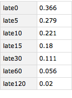
So, it turns out that in 2015 about 18% of flights were late by more than 15 minutes. 5.6% of flights were more than an hour late. But 63.4% of flights were on time or early.

Late Arrivals By Month

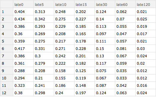
We can now determine these values for each month. Here I group the data by month and then treat each resulting piece the same as I treated the whole Dataset in the code immediately above.We wrap the results of our Query with a KeySort so that the months are in order. What we can see is that February and June are actually the worst months for delays and that October is probably the best month in which to fly (on average).

Query[GroupBy[#month &] /* KeySort, lateness[delays], Slot["arrival_delay"] &][ds]

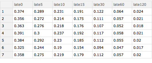
I can also determine how lateness varies according to the day of the week. The results show that Saturday is the best day to fly with Thursday generally being the worst.

Query[GroupBy[#"day_of_week" &] /* KeySort, lateness[delays], 
  Slot["arrival_delay"] &][ds]

Late arrivals by airport

Our Dataset uses airport codes instead of airport names. Often the latter is more convenient. I thus build a little Association that we can use to translate from 3-letter airport codes to airport names.

iatamap = Association[Rule @@@ Rest@iataCSV]

Here' s an example showing how our iatamap Association works.

iatamap["IAH"]

"Houston, TX: George Bush Intercontinental/Houston"

This same programming pattern can be used to compute the breakdown of lateness by originating airport. We'll only use airports that have more than 250 originating flights. To do this, I first group by "origin_airport" and then select only those groups that have more than 1000 rows associated with them. The code is then essentially the same as when I grouped by month.

byOriginAirport = 
 Query[GroupBy[#"origin_airport" &] /* Select[Length[#] > 1000 &] /* 
    KeySort, lateness[delays, ("origin_late" <> ToString[#] &)], 
   Slot["arrival_delay"] &][ds]

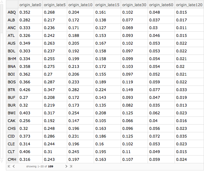
We can now produce a Dataset in which the origin airport is sorted according to the fraction of flights that are at least 15 minutes late and in which the origin airport is given its full name. I show the top 10 entries. We can see that the Hawaiian airports do well as does Akron, Ohio, Portland, Oregon and Salt Lake City, Utah. Anchorage, Alaska does surprisingly well given the sometimes challenging weather that prevails there.

Query[1 ;; 10][
 Query[SortBy[Slot["origin_late15"] &] /* KeyMap[iatamap]][
  byOriginAirport]]

And here are the ten worst origin airports: O'Hare, White Plains, New York, Baton Rouge and Dallas, Love Field.

Query[1 ;; 10][
 Query[SortBy[Slot["origin_late15"] &] /* Reverse /* KeyMap[iatamap]][
  byOriginAirport]]

We can also look at matters by destination airport. Again, the Hawaiian airports (LIH, KOA, ITO, OGG) do well, along with Salt Lake City.

byDestinationAirport = 
 Query[GroupBy[#"destination_airport" &] /* 
    Select[Length[#] > 1000 &] /* KeySort, 
   lateness[delays, ("destination_late" <> ToString[#] &)], 
   Slot["arrival_delay"] &][ds]

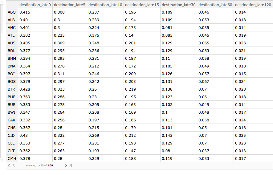
Here are the 10 best airports when serving as a destination. Again, many of the Hawaiian island airports do well. But so does Salt Lake City and Atlanta.

Query[1 ;; 10][
 Query[SortBy[Slot["destination_late15"] &] /* KeyMap[iatamap]][
  byDestinationAirport]]

The worst airports on the receiving end are Colorado Springs (snow?), Laguardia Airport, Little Rock, Fayetteville, Knoxville and White Plains. It is unclear why the two Arkansas airports have problems as the area is known neither for particularly bad weather or congestion.

Query[1 ;; 10][
 Query[SortBy[Slot["destination_late15"] &] /* Reverse /* 
    KeyMap[iatamap]][byDestinationAirport]]

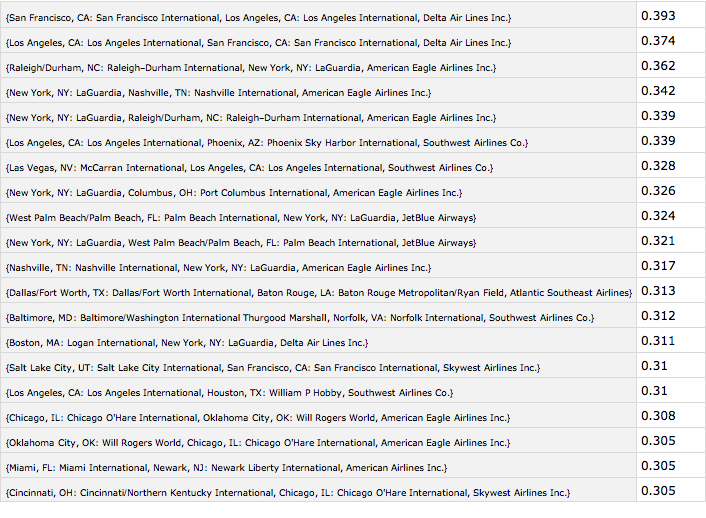
We can also find the worst routes by origin, destination and airline. I use some fancy formatting code so that the result is not too wide. It turns out Delta's flight from San Francisco to Los Angeles and the flight back from Los Angeles to San Francisco are the worst, running more than 15 minutes late over 37% of the time. Several American Eagle flights in and out of Laguardia also have serious problems as does Southwest Airlines flights between Los Angeles and Phoenix.

byOriginDestinationAirline = 
  Query[GroupBy[{#"origin_airport", #"destination_airport", \
#airlineName} &] /* Select[Length[#] > 200 &] /* KeySort, 
    lateness[delays], Slot["arrival_delay"] &][ds];

Query[(1 ;; 20) /* 
   KeyMap[Style[{iatamap[#[[1]]], iatamap[#[[2]]], #[[3]]}, 
      9] &], #"late15" &][
 Query[SortBy[#late15 &] /* Reverse][byOriginDestinationAirline]]

Comparison of lateness with airport as origin airport and airport as destination airport

We can also compare lateness as an originating airport with lateness as a receiving airport. The code here is a bit challenging. But observe. First we make the city a column of the dataset.

asOriginAndDestination = 
 Dataset[JoinAcross[
    KeyValueMap[Association[#2, "city" -> #1] &, 
     Normal[byOriginAirport]], 
    KeyValueMap[Association[#2, "city" -> #1] &, 
     Normal[byDestinationAirport]], "city"]][All, 
  KeyTake[#, {"city", "origin_late15", "destination_late15"}] &]

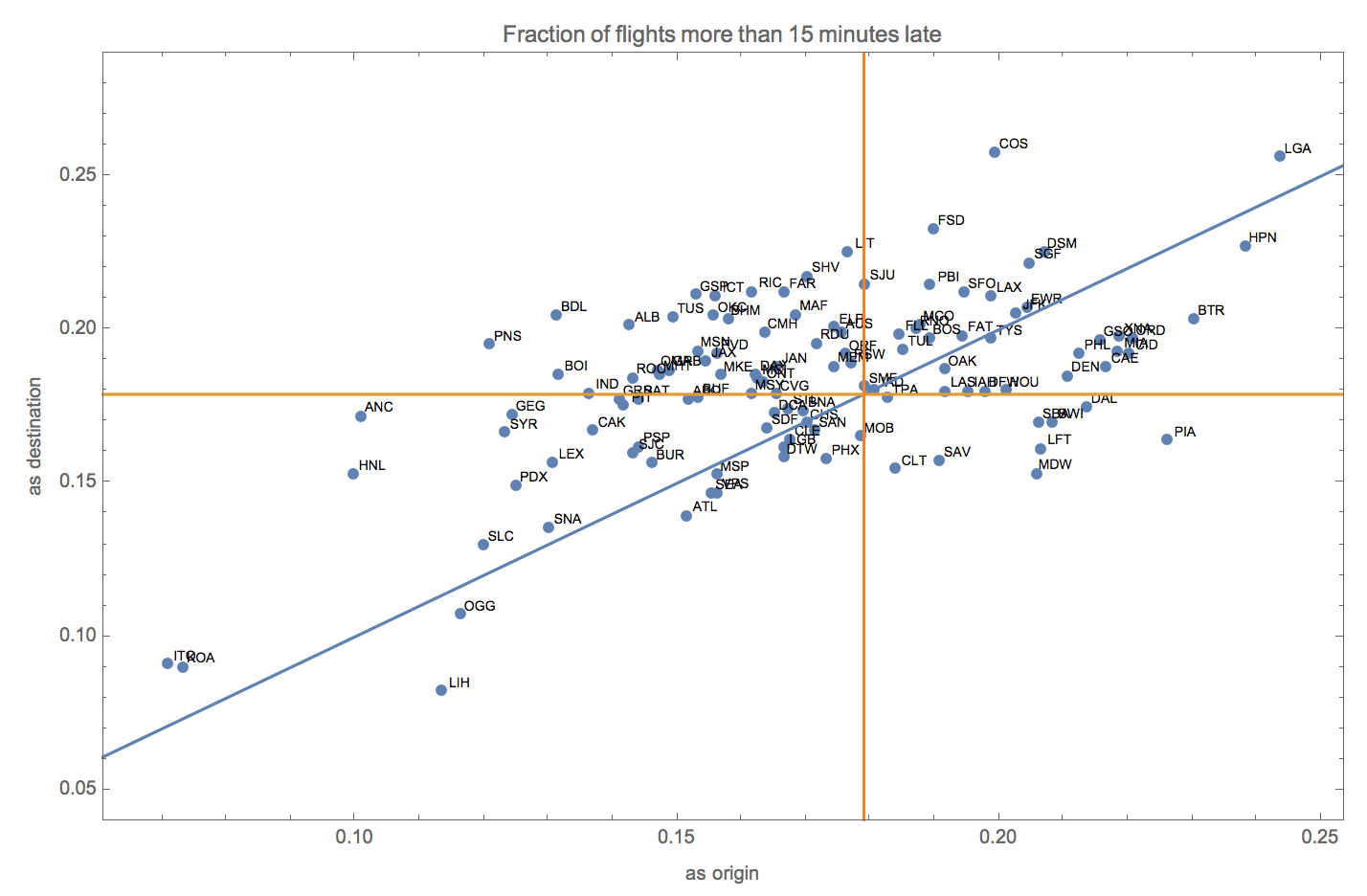
We can do something pretty fancy with this data. We can plot for each airport the fraction of flights that are more than 15 minutes late when it serves as an originating airport (x) versus the fraction of flights that are more than 15 minutes late when it serves as a destination airport (y). The points are labeled with the associated airport. One can superimpose on this graphic lines showing the mean number of flights late by more than 15 minutes. Flights in the northeast quadrant of the plot such as LGA (Laguardia) and DEN (Denver) are worse than average. Flights above the blue line such as COS (Colorado Springs) or SFO (San Francisco) are worse as a destination airport than as an origin airport. Flights below the blue line such PHL (Philadelphia) and BTR (Baton Rouge) are worse as an origin airport than as a destination airport. Flights in the northwest quadrant such as BDL (Bradley in Hartford Connecticut) and ALB (Albany, New York) are worse than average as a destination airport but better than average as an origin airport. Flights in the southwest quadrant such as ANC (Anchorage, Alaska) and ATL (Atlanta) are better than average both as a origin and destination airport. And the few flights in the southeast quadrant such as CLT (Charlotte, North Carolina) and MDW (Midway, Chicago) are worse than average as an origin airport but better than average as a destination airport. One can also see from this graphic that the Hawaiian island airports dominate in terms of avoiding both arrival delays whether serving as the originating or destination airport.

Module[{data = Normal[asOriginAndDestination[All, Values]], lp, g},
 lp = ListPlot[Part[data, All, {2, 3}], Axes -> False, Frame -> True, 
   FrameLabel -> {"as origin", "as destination"}, 
   PlotRange -> {0.05, 0.28}, 
   PlotLabel -> "Fraction of flights more than 15 minutes late", 
   PlotRangePadding -> 0.01];
 g = Graphics[
   Map[Text[Style[#[[1]], 7], {#[[2]] + 0.003, #[[3]] + 0.002}] &, 
    data]];
 Show[lp, g, Plot[{x, 0.17898}, {x, 0, 1}], 
  Graphics[{Orange, InfiniteLine[{{0.17898, -10}, {0.17898, 10}}]}]]

 ]

Lateness by Time of Scheduled Departure

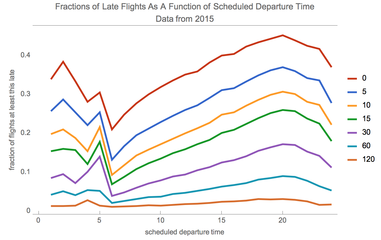
Let' s find out how lateness in arrival depends on the scheduled time of departure. We can use similar code to that we used to see how lateness varies by month. We can extract the departure hour using the DateValue function with "Hour" as its second argument.

arrivalDelayByScheduledDepartureTime = 
 Query[GroupBy[DateValue[#"scheduled_departure_time", "Hour"] &] /* 
    KeySort, lateness[delays], Slot["arrival_delay"] &][ds]

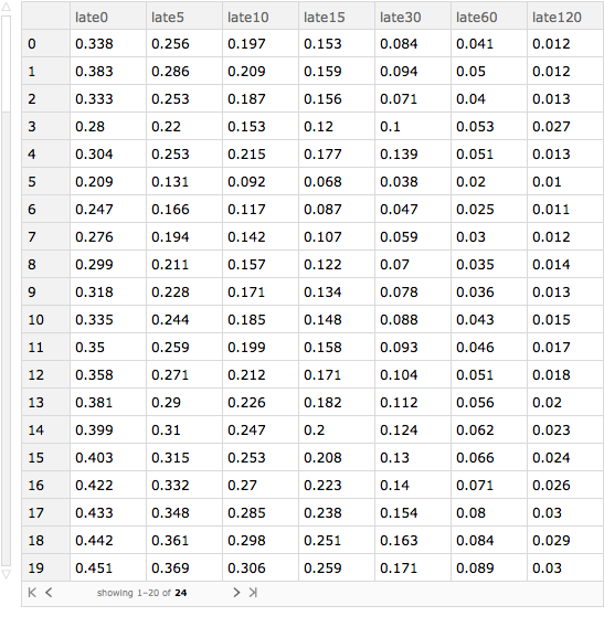Let' s plot the result.

figureScheduledDeparture = 
 With[{plottingFunction = (ListLinePlot[#, Axes -> False, 
       Frame -> True, 
       FrameLabel -> {"scheduled departure time", 
         "fraction of flights at least this late"}, 
       PlotLegends -> delays,
       PlotLabel -> 
        "Fractions of Late Flights As A Function of Scheduled \
Departure Time\nData from 2015", ImageSize -> 600, BaseStyle -> 12, 
       PlotTheme -> "Web"] &)}, 
  Transpose[arrivalDelayByScheduledDepartureTime][
   Values /* plottingFunction, Values]
  ]

So, time of day matters for scheduled departure matters hugely in determining whether one is going to be late or not. Flights leaving at 5 or 6 in the morning are far more likely to be on time than flights leaving at around 8 p.m., by which time prior delays have cascaded.

Analysis By Airline

Now, let' s see how lateness varies by airline. Again, most of our coding work is done. We just have to change how we group the data.

arrivalDelayByAirline = 
 KeySort[Query[GroupBy[#"airlineName" &], lateness[delays], 
    Slot["arrival_delay"] &][ds]]

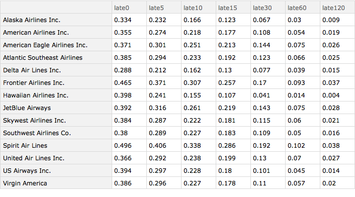
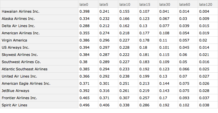
I now sort the data according to whether the flights were more than 15 minutes late. We can see there is a big difference. Hawaiian Airlines does best, perhaps owing to our 50th state's generally fabulous weather, but Alaska Airlines does extremely well too, even though many of its flights go into more challenging destinations. Spirit Airlines (a budget carrier) and Frontier Airlines (also sometimes regarded as a budget carrier) do worst. Of the major carriers, Delta does best by a significant margin and United Airlines does worst. The ordering does not vary greatly based on which particular lateness metric one uses.

arrivalDelayByAirlineSorted = 
 Query[SortBy[#late15 &]][arrivalDelayByAirline]

Let' s also try something of possible interest. Let' s first find the 10 most busy origin airports.

busyAirports = 
 Query[GroupBy[#"origin_airport" &] /* Sort /* 
    Reverse /* (Take[#, UpTo[10]] &), Length][ds]

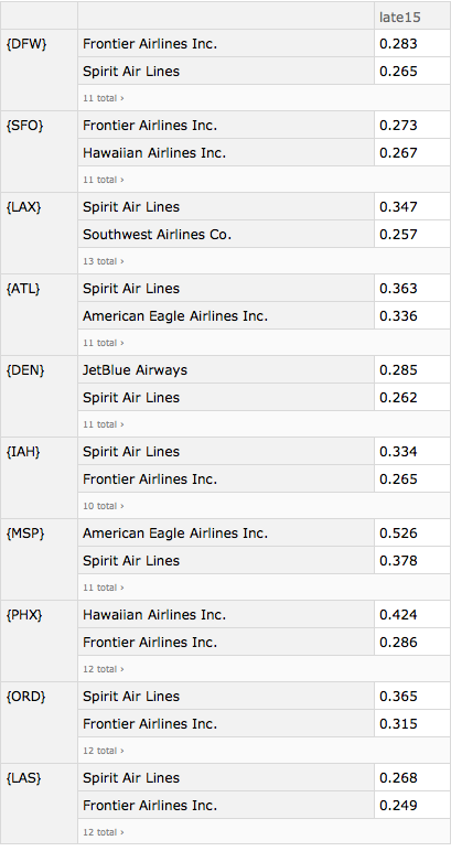
Now let' s see how the airlines rank when their flights originate from these airports. This will be our most complicated analysis. First let's get the most busy airports, filter our dataset down to those airports and then group the data by airport. We'll then group each of the airports by airlines and for each calculate the fraction more than 15 minutes late. We'll sort each of the airports by the lateness fraction from worst to best.

busyAirportKeys = Normal@Keys@busyAirports

complexQuery = 
 Query[(Select[
     MemberQ[busyAirportKeys, #"origin_airport"] &]) /* \
(GroupBy[{#"origin_airport"} &]), 
  GroupBy[#airlineName &] /* ReverseSort, lateness[{15}], 
  Slot["arrival_delay"] &]

byOriginAirportAndAirlineLateness = complexQuery[ds]

We can now print out the results for each of the airports.

Column@Table[
  Framed[Labeled[byOriginAirportAndAirlineLateness[i], 
    First@Normal@Keys[byOriginAirportAndAirlineLateness][[i]], 
    Top]], {i, Length[byOriginAirportAndAirlineLateness]}]

The results show immense variation in lateness even when the departure airport is the same. Hubness matters. From Houston's Bush Intercontinental Airport (IAH), for example, Spirit Airlines is late 33.4% of the time whereas the large American Airlines is late only 14.8% of the time. In Atlanta, United is late 21.3% of the time whereas Delta is late only 12.7% of the time. In Denver, Alaska Airlines is late only 11.1% of the time whereas JetBlue is late 28.5% of the time.

Conclusions

Mathematica can handle large datasets reasonably well.

You can learn a lot about airline performance based on the Kaggle 2015 dataset.