President Trump will evidently propose today (10/12/2017) some expansion of alternative health insurance arrangements such as "short term health insurance" or "Association Health Plans." Supporters say this proposal will give more Americans the chance to buy health insurance policies at lower prices and that better fit their needs. Critics say that this expansion will result in healthier people deserting insurance plans in which the price can not depend on the expected claims of the individual. This desertion will in turn cause expected claims in the original pool to rise, leading to insurers losing money and raising prices.

Can Mathematica quantify this possibility? Thus, a little quick experiment.

I start with a reparameterized version of the lognormal distribution in which the first parameter is the mean and the second parameter is the ratio of the median to the mean.

LogNormalDistribution3[m_,?_]:=LogNormalDistribution[Log[m]-Log[1/?],Sqrt[2] Sqrt[Log[1/?]]]

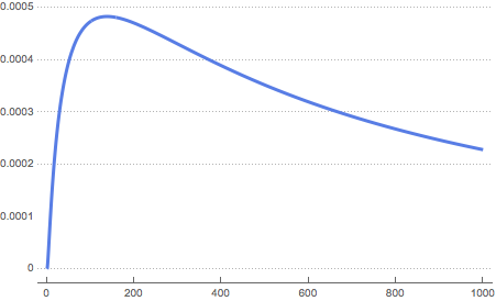
Here is probability density function for the values of parameters used below:

Plot[PDF[LogNormalDistribution3[7000, 0.27], x], {x, 0, 10^3}, PlotTheme -> "Business"]

I now create a risk pool with 100, 000 persons with mean claims of 7,000 and a ratio of median to mean of 0.27. This models fairly well the current situation. The actual selection of the mean does not affect the results. The median to mean ratio does affect results, however.

rv = RandomVariate[LogNormalDistribution3[7000, 0.27], 100000]

Now, create a function that computes the mean claims of those not defecting to an alternative pool when those with expected claims below the median have a specified probability of defecting to the alternative pool. We could create a more general defection function that made the probability of defection depend inversely on the expected claims of the individual, but this approach strikes me as reasonable for a quick and dirty analysis.

residualExpectedClaims[rv_,defectionProbability_]:=Mean@Pick[rv,
With[{median=Median[rv]},Map[If[#<median,RandomVariate[BernoulliDistribution[1-defectionProbability]],1]&,rv]],1]

Now let's run an experiment in which 25% of those below the median defect.

r025 = residualExpectedClaims[rv, 0.25]

We can now compute the fractional increase in risk in the original pool.

(r025-Mean[rv])/Mean[rv]

The answer is about 13%.

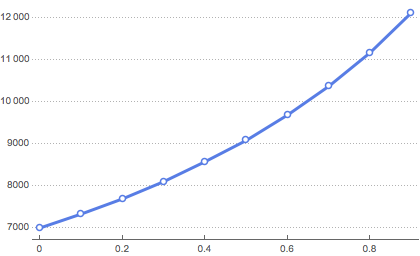
We can also make a table showing how the residual expected claims vary as the fraction of defectors increases:

originalPoolExpectedClaims=Table[{defectPct,residualExpectedClaims[rv,defectPct]},{defectPct,0,0.9,0.1}]

Here's the output:

{{0., 7000.}, {0.1, 7322.07}, {0.2, 7684.62}, {0.3, 8111.13}, {0.4, 8552.09},

{0.5, 9061.95}, {0.6, 9677.75}, {0.7, 10359.4}, {0.8, 11146.6}, {0.9, 12142.1}}

ListLinePlot[originalPoolExpectedClaims, PlotTheme -> "Business"]

There's obviously more that can be done, but I thought Mathematica did a great job here in quickly modeling out the consequences of what may be a very important policy change in the United States.

Closed form solution

It turns out there is a closed form solution to the problem I originally posed and for which I originally simulated results. I present it here.

Recall that the project is to determine the ratio between the expected values (means) of two distributions: an original distribution and a post-defection distribution. The original distribution represents the health insurance claims filed by a pool of insureds. It is described as a lognormal distribution that has a mean of m and a ratio between its median and its mean of v. One can think of v as a measure of the heterogeneity of claims. Low v means claims are highly heterogeneous; high v means the distribution is more symmetric and that claims are fairly homogeneous.

LogNormalDistribution3[m_, \[Nu]_] := 
 LogNormalDistribution[Log[m] - Log[1/\[Nu]], 
  Sqrt[2] Sqrt[Log[1/\[Nu]]]];
original = LogNormalDistribution3[m, v];

The idea of the post-defection distribution is that, because of hypothesized implementations of an Executive Order signed today by President Trump, some fraction of those below the median level of claims might purchase alternative forms of insurance. We can describe the post-defection distribution as a mixture distribution in which the weights are a and 1-a. The components are both truncated distributions, the first being right-truncated at the median and the second being left-truncated at the median.

postDefection = 
 MixtureDistribution[{a, 
   1 - a}, {TruncatedDistribution[{0, m*v}, original], 
   TruncatedDistribution[{m*v, \[Infinity]}, original]}]

We can now compute the mean of the post-defection distribution. The output is called ratio. Warning: this may take up to 10 minutes, depending on one's computer. Apparently, the underlying integral is somewhat complex.

ratio = FullSimplify[
  Refine[Mean[postDefection], 0 < a < 1 && m > 0 && 0 < v < 1]/m]

The result is:

$$(2 a-1) \text{erfc}\left(\sqrt{-\log (v)}\right)-2 a+2$$

What we see is that the mean m has dropped out and that the ratio depends simply on the weighting a placed on those with claims less than the median and v the heterogeneity of the original distribution.

I would prefer to describe the scenario not in terms of weights attached to those with claims less than the median but rather with a fraction b of those with claims below the median that will defect to alternative forms of insurance due to implementations of the Trump executive order. This can be done with a reparameterization rule:

reparameterizationRule = a -> ((1 - b)*(1/2))/((1 - b)*(1/2) + 1/2);
FullSimplify[ratio /. reparameterizationRule]

The result is

$$\frac{b \text{erfc}\left(\sqrt{-\log (v)}\right)-2}{b-2}$$

We can thus write our final function meanRatio that yields the desired result:

meanRatio[v_, b_] :=  (-2 + b*Erfc[Sqrt[-Log[v]]])/(-2 + b)

If we set v=0.27 and b=0.25 -- which was what was done in the original simulation -- we obtain 1.12777, which is extremely close to the simulated result. If 25% of those with claims below the median defect to alternative forms of insurance, the mean claims of those remaining in the original pool goes up about 13%.

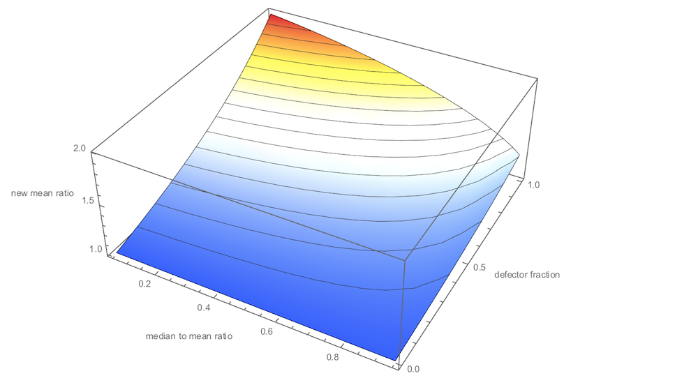
The code below produces a surface showing how different values of v and b determine the ratio of mean claims post defection to original mean claims.

Plot3D[meanRatio[v, b], {v, 0.05, 0.95}, {b, 0, 1}, 
AxesLabel -> {"median to mean ratio", "defector fraction", "new mean ratio"}, 
ImageSize -> 600, ColorFunction -> "TemperatureMap", MeshFunctions -> {#3 &}]

Attachments: