Building on Gianluca's ideas, one can do two things, separate out further the smallest bit of the computation that depends on the dynamic variable t and manually construct a mesh that efficiently represents the plot (rather than use DensityPlot's rectangular mesh, which is rather awkward for this plot).
Needs["NDSolve`FEM`"];

rate = 3;  (* can set it to 2 for a smaller mesh *)
npts = rate * 40; (* number of steps in the spiral lines *)
nlines = 15;  (* can set it to 10 for a smaller mesh *)
z0 = Exp[(-0.1 + 0.5 I )/rate];
bmesh = ToBoundaryMesh["Coordinates" -> Join[
     {{-25., -25.}, {25., -25.}, {25., 25.}, {-25., 25.}},
     ReIm@
      Flatten@NestList[Exp[I*2 Pi/nlines]*# &,
        NestList[z0*# &, 23., npts - 1], nlines - 1]
     ],
   "BoundaryElements" -> Join[
     {LineElement[{{1, 2}, {2, 3}, {3, 4}, {4, 1}}]},
     Table[LineElement[Partition[4 + k*npts + Range@npts, 2, 1]],
      {k, 0, nlines - 1}]
     ]
   ];
emesh = ToElementMesh[bmesh]
Show[
 emesh["Wireframe"],
 emesh["Wireframe"["MeshElement" -> "BoundaryElements",  "MeshElementStyle" -> Red]]
 ]
gc = First@Cases[emesh["Wireframe"], _GraphicsComplex, Infinity];
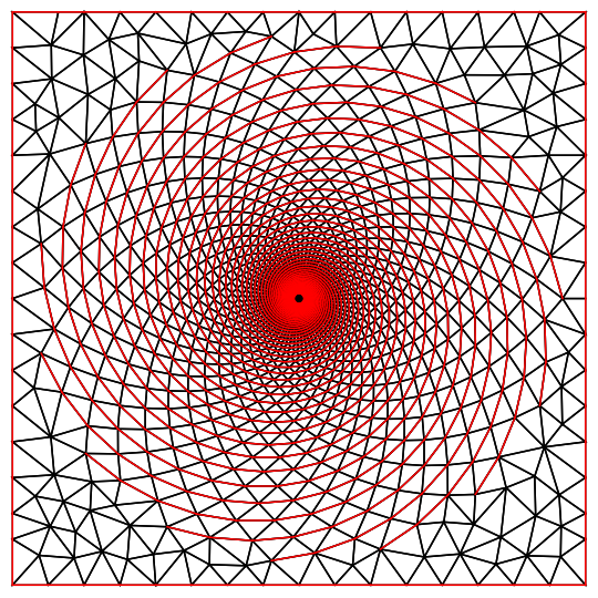
It has almost 8000 points. You probably don't want it to get too much above 10000.
emesh["Coordinates"] // Length
(*  7817  *)
Then
Clear[g0];
g0[t_] := Exp[(-Cos[2*(a - t) + (2/(Tan[7*Pi/90]))*Log[r/4.9]])];
With[{array = {ArcTan[#[[1]], #[[2]]], Sqrt[#[[1]]^2 + #[[2]]^2]} &@
Transpose@First@gc},
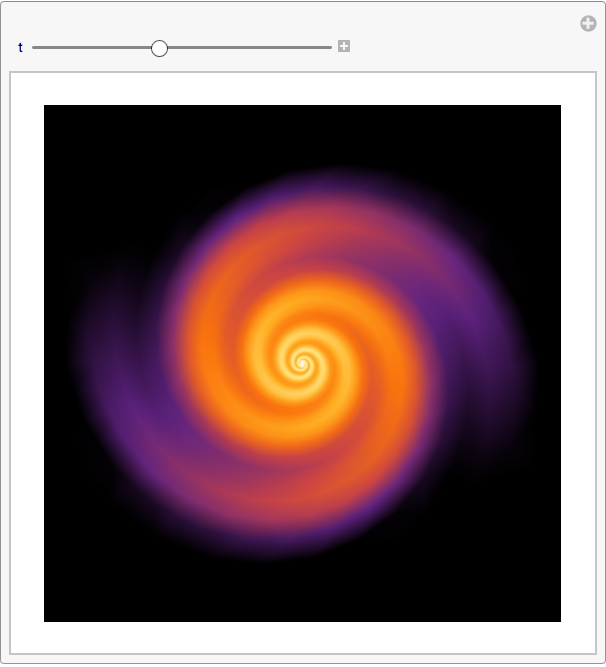
Manipulate[
Graphics[
Append[
gc,
VertexColors ->
Dynamic[ColorData["SunsetColors"] /@
LogarithmicScaling[(scale*(g0[t] /. Thread[{a, r} -> array]) +
offset), 10.^1, 10.^5
]]
]
],
{t, 0, 10},
{{offset, +7.013941065*10^5*interp[r^2] +
Integrate[(7.321354473)/(1 + (Sqrt[r^2 + z^2]/3.936)^2)^(5/2), {z, -Infinity, +Infinity},
Assumptions -> r^2 >= 0] /.
Thread[{a, r} -> array]}, None},
{{scale,
2.872416767*10^3*Exp[(-r)/2.676]*Exp[(1)] * Integrate[Exp[-Abs[z]], {z, -Infinity, +Infinity}] /.
r -> Last@array}, None}
]
]