Introduction
Elections are fundamental to our democracies and way of life. The electorate bestows power on the lawmakers and public officials whose legitimisation is derived solely from the fact that they are elected. In recent times, many elections, such as the presidential elections the United States and the Brexit and general elections in the United Kingdom have seen a very pronounced polarisation the electorate. Can mathematics and the Wolfram Language help to better understand this crucial process of the most fundamental decision making process in societies? The main question I want to discuss in a sequence of posts is what can be learnt from elections. So this post is about computational politics. It is important to notice that democracies rely on a general acceptance of the result of elections. Without that consensus a peaceful co-existence is at risk. Societies agree on certain electoral procedures and the results have to be understood to be final. There are, however, more fundamental questions such as how do we derive the "voters will" from ballots. That is a highly non-trivial problem. Also, elected politicians often claim that they represent the "will of the people". But is that true and what is the "will of the people"? Hence, my question: the voters have spoken - but what did they say?
This is the second of a series of posts (hopefully):
- Electoral systems - interpreting the will of the voters
- Gerrymandering - shaping the voters' will to your liking
- Analysis of the Brexit vote - how do we know what did the voters really want?
In the following posts we will apply some more sophisticated algorithms to try to figure out what the voters meant to tell us. We will then see that we can use mathematics to estimate what the voters might have wanted to tell us; and then we can correct for that.
Note, that this cannot be the procedure by which we determine the decision that the electorate have taken. This is all a bit confusing, but I hope that it will become a bit clearer in these posts. All posts were developed with Bjoern Schelter, who is also a member of this community. We could also like to thank @Brian Wood , @Vitaliy Kaurov , @Danielle Rommel , and @Karenna Lange for their help and useful discussions. This part will discuss the issue of Gerrymandering.
Gerrymandering
Gerrymandering is currently being discussed widely. Here is the definition from Wikipedia
Style[StringJoin["        ", StringTake[
StringReplace[WikipediaData["Gerrymandering"], "\n" -> " "], 1091]], 16, FontFamily -> "American Typewriter"]

The etymology of the term is also interesting:
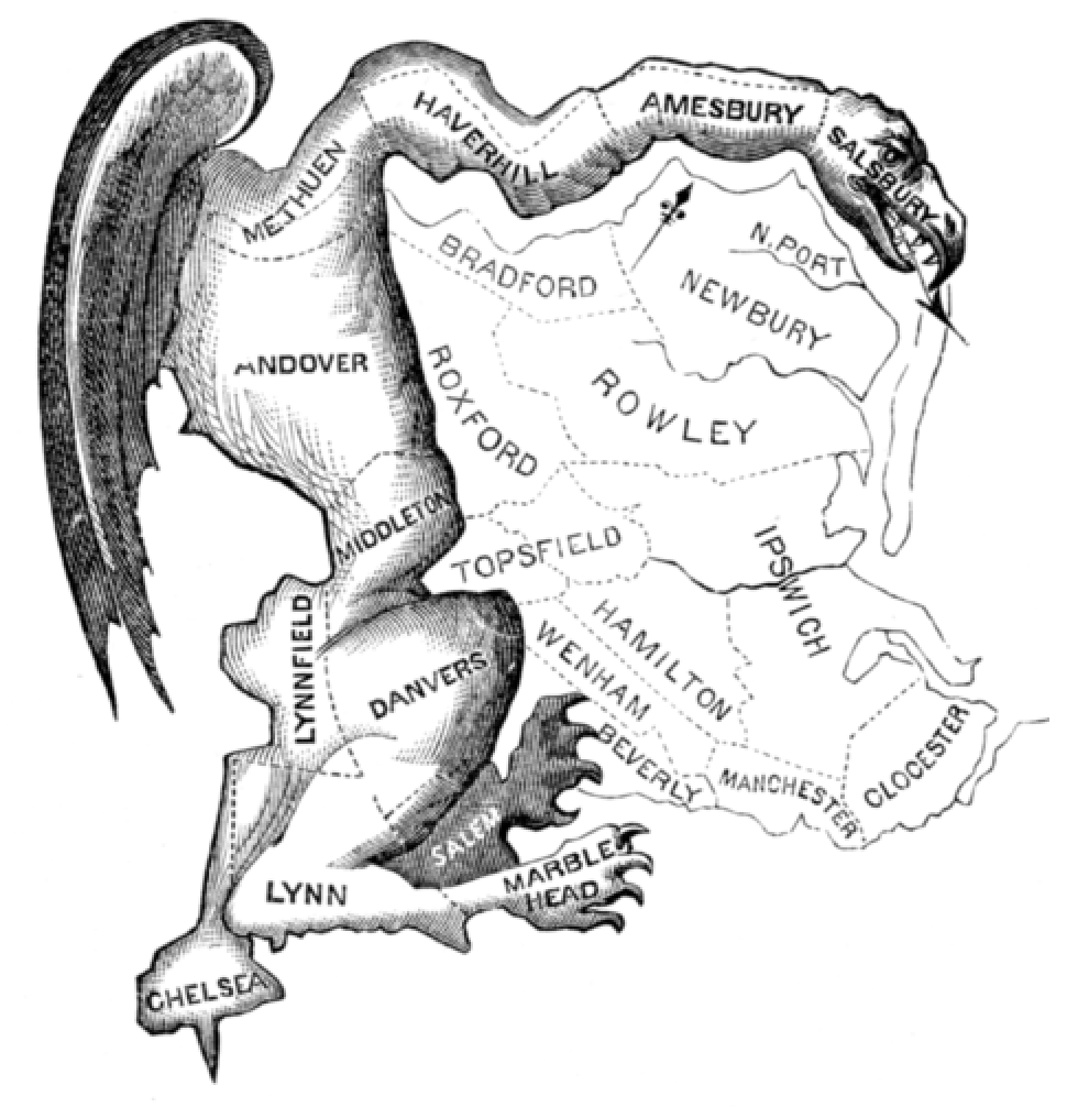
"The word gerrymander (originally written Gerry-mander) was used for the first time in the Boston Gazette on 26 March 1812. The word was created in reaction to a redrawing of Massachusetts state senate election districts under Governor Elbridge Gerry (pronounced /???ri/; 1744[Dash]1814). In 1812, Governor Gerry signed a bill that redistricted Massachusetts to benefit his Democratic-Republican Party. When mapped, one of the contorted districts in the Boston area was said to resemble the shape of a mythological salamander." (Wikipedia)
This is the famous image from the Boston Gazette:
There is a documentary about gerrymandering that might be worth watching. (I haven't finished watching it though.)
First example of Gerrymandering
The fact that in indirect elections voting outcomes can be changed by adjusting boundaries of electoral districts can be visualised.
GraphicsRow[{Graphics[
   Flatten[Join[Flatten[Join[{EdgeForm[Gray], FaceForm[Green]},
   Flatten[Table[Rectangle[{i, j}], {i, 1, 2}, {j, 1, 10}], 1]], 1], Flatten[Join[{EdgeForm[Gray], FaceForm[Red]},
   Flatten[Table[Rectangle[{i, j}], {i, 3, 5}, {j, 1, 10}], 1]], 1]], 1],
   Epilog -> Flatten[{Black, Thickness[0.02], Line /@ Table[{{1, k}, {5.98, k}}, {k, 1, 11, 2}], Line[{{5.98, 1}, {5.98, 11}}], Line[{{1, 1}, {1, 11}}]}, 1]],
 Graphics[Flatten[Join[Flatten[Join[{EdgeForm[Gray], FaceForm[Green]}, Flatten[Table[Rectangle[{i, j}], {i, 1, 2}, {j, 1, 10}], 1]], 1], Flatten[Join[{EdgeForm[Gray], FaceForm[Red]}, Flatten[Table[Rectangle[{i, j}], {i, 3, 5}, {j, 1, 10}], 1]], 1]], 1],
   Epilog -> Flatten[{Black, Thickness[0.02],
      Line /@ {{{1, 1}, {2, 1}}, {{2, 1}, {2, 2}}, {{2, 2}, {5, 2}}, {{5, 2}, {5, 5}}, {{5, 4}, {2, 4}}, {{2, 4}, {2, 5}}, {{2, 5}, {1, 5}}, {{5, 5}, {3, 5}}, {{3, 5}, {3, 7}}, {{3, 6}, {5.98, 6}}, {{3, 7}, {5, 7}}, {{5, 7}, {5, 10}}, {{5, 8}, {2, 8}}, {{2, 8}, {2, 7}}, {{2, 7}, {1, 7}}, {{5, 10}, {2, 10}}, {{2, 10}, {2, 11}}, {{2, 11}, {1, 11}}, {{5.98, 1}, {5.98, 11}}, {{1, 1}, {1, 11}}, {{1, 1}, {5.98, 1}}, {{1, 11}, {5.98, 11}}}}, 1]]}]
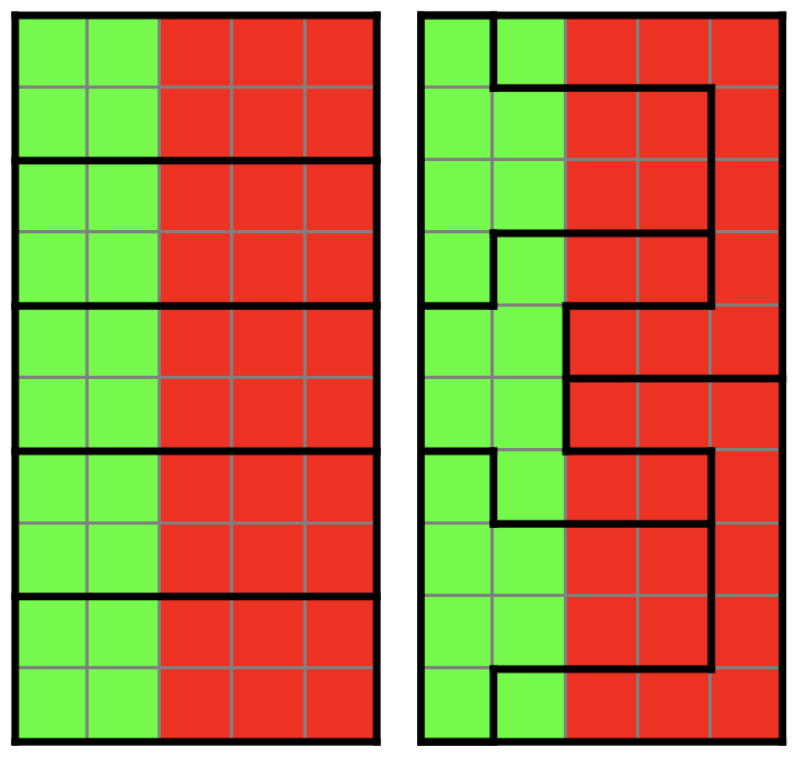
Each box represents one voter; the colours indicate voting preference. There are 20 voters in favour of "green" and 30 voters in favour of "red". The left panel shows district boundaries such that all districts would be won by red. The right panel shows alternative district boundaries. Now two districts are won by red (with 100% of the votes for red) and three districts are won by green. Which would give the representatives of green a majority. Note that the voting preferences are the same in both cases, but the winner (social choice) is different. This begs two questions: (i) is there a "good" algorithm for choosing boundaries of electoral districts, and (ii) is it possible to detect instances of gerrymandering?
Data acquisition and preparation
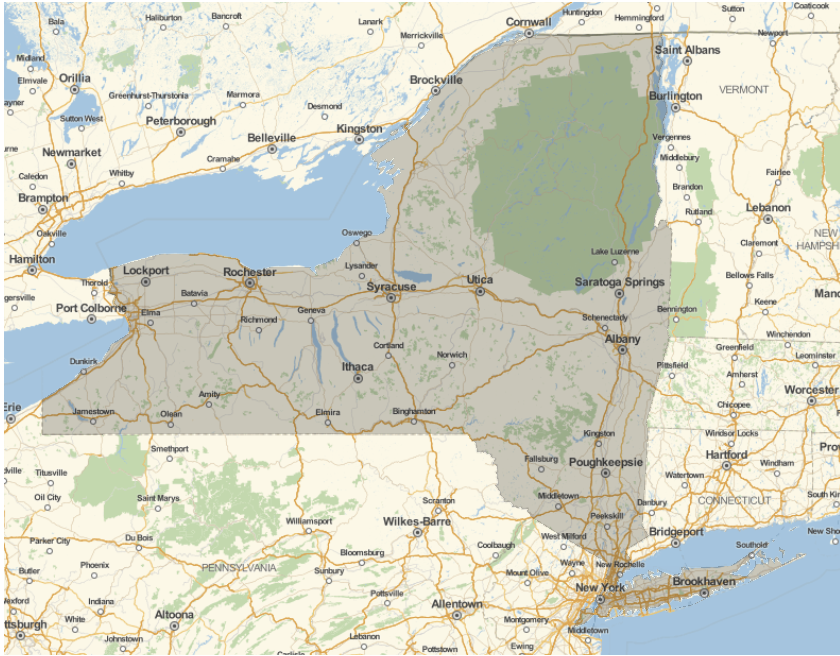
We will first acquire some data that will be useful for the remaining post. We first note that the Wolfram Language has much of the data we need already built in. We will need the polygonal outline of different states and they are readily available like so:
GeoGraphics[Entity["AdministrativeDivision", {"NewYork", "UnitedStates"}]["Polygon"]]
We will also use some data from this website. I particular we will need the files: cb2016uscd115500k.zip, cb2016uscd1155m.zip, and cb2016uscd11520m.zip. Let's import some of the data (assuming that the relevant subfolders are in the same directory as this notebook):
SetDirectory[NotebookDirectory[]];
districtsUS = Import["cb_2016_us_cd115_5m/cb_2016_us_cd115_5m.shp", "Data"];
There are
Length[districtsUS[[1, 2, 2]]]
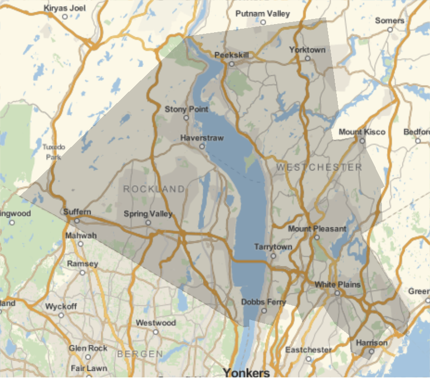
441 electoral districts. Here is the 8th from the end:
GeoGraphics[districtsUS[[1, 2, 2]][[-8]]]
We will also generate "polygon codes", which are sets of two numbers: the first for the state and he second for the district.
polygoncodes = StringPartition[#, 2] & /@ (districtsUS[[1, -2 ;;, 2, 4]][[2, 2]]);
Next we generate a list with the codes for the states:
stateCodes =
 Join[#[[2]] -> #[[3]] & /@ SortBy[Partition[Flatten[Import["https://www.mcc.co.mercer.pa.us/dps/state_fips_code_listing.htm", "Data"][[1, 2 ;;]]], 3], #[[2]] &], {"69" -> "Northern Marianna Islands"}]

So if we want all electoral districts from Oklahoma (40) we use:
Select[polygoncodes, #[[1]] == "40" &]
(*{{"40", "04"}, {"40", "03"}, {"40", "02"}, {"40", "01"}, {"40", "05"}}*)
Let's plot the districts for, say New York:
newYorkdistricts = Flatten[Position[polygoncodes, #] & /@ Select[polygoncodes, #[[1]] == "36" &]];
styling = {GeoBackground -> GeoStyling["StreetMapNoLabels", GeoStylingImageFunction -> (ImageAdjust@
ColorNegate@ColorConvert[#1, "Grayscale"] &)], GeoScaleBar -> Placed[{"Metric", "Imperial"}, {Right, Bottom}],
   GeoRangePadding -> Full, ImageSize -> Large};
ImageAdd[GeoGraphics[Entity["AdministrativeDivision", {"NewYork", "UnitedStates"}], styling],
GeoGraphics[Riffle[RandomColor[Length[newYorkdistricts]], districtsUS[[1, 2, 2]][[newYorkdistricts]]], GeoBackground -> None]]
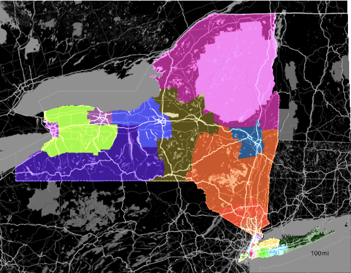
This is basically all the data that we need. In the next section, we will develop a simple algorithm that is not very efficient and will have some flaws, but that will show how in principle the partitioning into districts can be performed in a "fairer" way.
Idea behind the partitioning algorithm
I will first walk you through the general idea behind the algorithm; later we will develop functions that can be used to actually perform the partitioning. Let us start with a region and voters (points) in it at random positions.
data = RandomPoint[Triangle[], 100];
Graphics[{LightGray, Triangle[], Red, Disk[#, 0.005] & /@ data}]
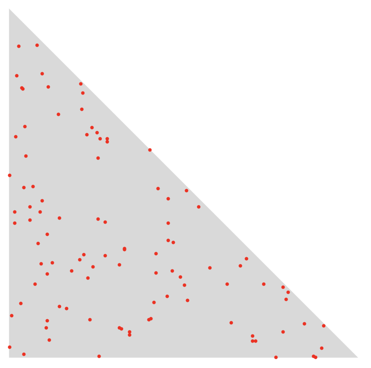
The objective is to split the region (triangle) into two subregions that contain the same number of points; if the number of points is odd, we will allow the regions to have a difference of one member. We also want to choose the shortest of all split lines. The first thing we will do is to compute a disk that contains all points:
boundingcircle = List @@ BoundingRegion[data, "MinDisk"]
(*{{0.45284, 0.446591}, 0.61426}*)
This can be visualised like so:
Graphics[{LightGray, Triangle[], LightGreen, Disk @@ boundingcircle, Red, Disk[#, 0.005] & /@ data}]
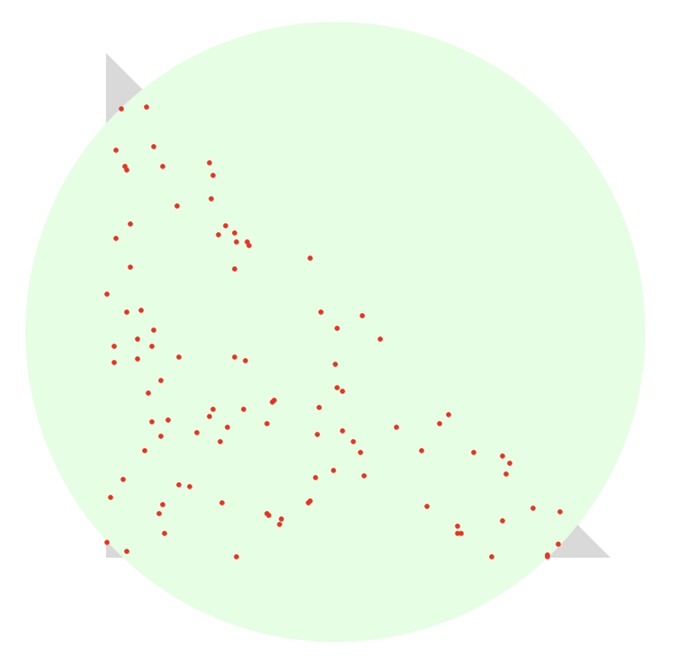
Next, we implement a function that increases the radius of the circle by 10% and calculates points on its surface (wrt to its origin):
pointsonpluscircle[p_] := 1.1 boundingcircle[[2]] {Cos[p], Sin[p]}
Then, we compute vectors perpendicular to the tangent at the boundary:
radiusperpendicular[p_] := RotationMatrix[Pi/2].{Cos[p], Sin[p]}
We then project all the data points onto the line perpendicular to the radius and calculate their median:
lengthprojection[p_] := Median[radiusperpendicular[p].(# - boundingcircle[[1]]) & /@ data]
and plot
Plot[lengthprojection[p], {p, 0, 2 Pi}]
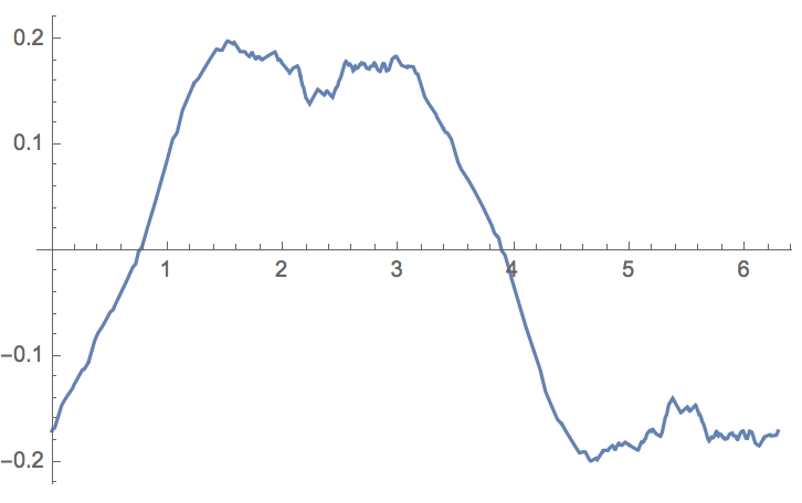
The idea is that we obtain the distribution of points along the tangent to a point on the radius. The median tells us by how much we have to translate a line perpendicular to the tangent so that the cloud of points is split into two subsets of equal size. So for a given angle (on the x-axes of the figure above), we obtain a shift along the tangent. Let's implement that into a function:
linesplit[theta_] := {#, # - 2*pointsonpluscircle[theta]} &@(pointsonpluscircle[theta] + boundingcircle[[1]] + lengthprojection[theta]*radiusperpendicular[theta])
For a given angle (here 0.33) we can now plot the splitline.
Show[Graphics[Line@linesplit[0.33]], Graphics[BoundingRegion[data, "MinDisk"] /. {Disk[{x_, y_}, r_] -> Circle[{x, y}, 1.1 r]}],
 Graphics[Join[{Red}, Point /@ data]]]
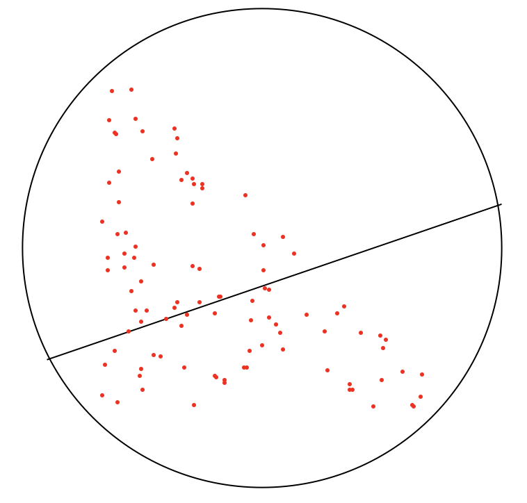
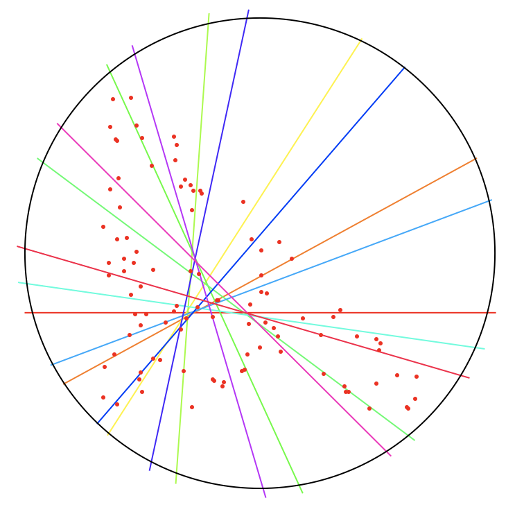
Our next step is to calculate all splitlines, i.e. for different angles, and then choose the shortest one inside the triangle:
Show[Graphics[Riffle[Table[Hue[theta/(2 Pi)], {theta, 0, 2 Pi, 0.5}], Line /@ Table[linesplit[theta], {theta, 0, 2 Pi, 0.5}]]],
 Graphics[BoundingRegion[data, "MinDisk"] /. {Disk[{x_, y_}, r_] -> Circle[{x, y}, 1.1 r]}],
 Graphics[Join[{Red}, Point /@ data]]]
Let's increase the lengths of the lines a bit:
linesplitlong[theta_] := {# + 3*pointsonpluscircle[theta], # - 3*pointsonpluscircle[theta]} &@(pointsonpluscircle[theta] +
boundingcircle[[1]] + lengthprojection[theta]*radiusperpendicular[theta])
and calculate the intersections with the triangle:
Show[Graphics[Triangle[]],
Graphics[Join[{Red}, RegionIntersection[Triangle[], #] & /@ (Line /@ Table[linesplitlong[theta], {theta, 0, 2 Pi, 0.01}])]]]

Now, all of the lines split the cloud of points into to halves. We next have to find the shortest of those lines:
Show[Graphics[Triangle[]], Graphics[Join[{Red}, Point /@ data]],
Graphics[{Yellow, MinimalBy[Table[{theta, RegionIntersection[Triangle[], #] &@Line[linesplitlong[theta]]}, {theta, 0, 2 Pi, 0.01}], ArcLength[#[[2]]] &][[1, 2]]}]]
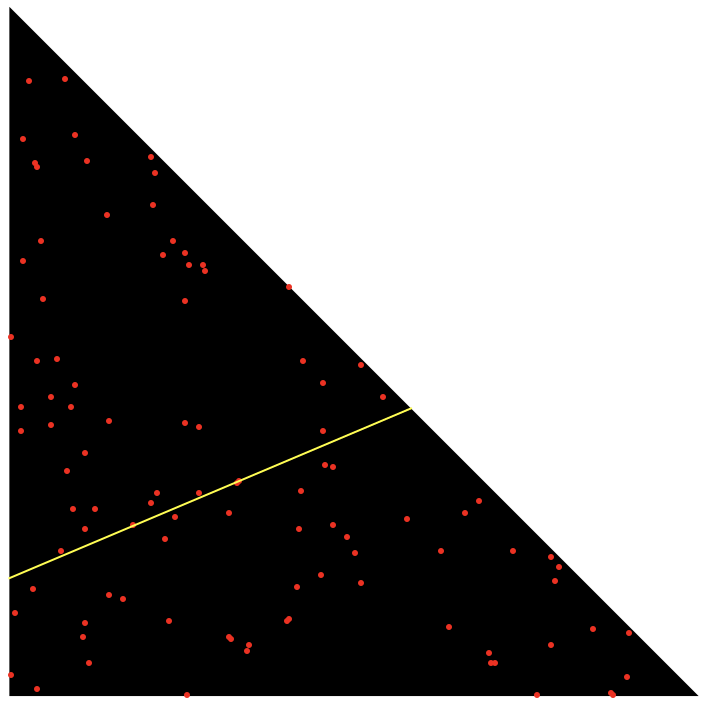
This would represent a "fair" split of the triangular region into two electoral subdistricts. The exact line is calculated like so:
splitline = MinimalBy[Table[{theta, RegionIntersection[Triangle[], #] &@
Line[linesplitlong[theta]]}, {theta, 0, 2 Pi, 0.01}], ArcLength[#[[2]]] &][[1, 2]]
(*Line[{{0.582629, 0.417371}, {-4.44089*10^-16, 0.17104}}]*)
We can then split the triangular region into two subregions:
Clear[r];
r1[point1_, point2_] := ImplicitRegion[{x, y} \[Element] Triangle[] && y >= point2[[2]] + (point2[[2]] - point1[[2]])/(point2[[1]] -
point1[[1]]) (x - point2[[1]]), {x, y}]
r2[point1_, point2_] := ImplicitRegion[{x, y} \[Element] Triangle[] && y <= point2[[2]] + (point2[[2]] - point1[[2]])/(point2[[1]] -
point1[[1]]) (x - point2[[1]]), {x, y}]
Show[RegionPlot[r1 @@ splitline[[1]]], RegionPlot[r2 @@ splitline[[1]]], PlotRange -> All]
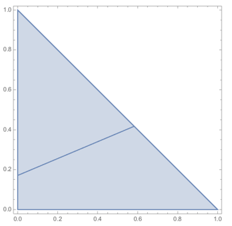
There are still a couple of issue with this. For example if there is an odd number of points, the line will go through one of the points. We need to fix this by slightly moving the line towards the point closest to the median. Also, as it turns out, it is not ideal to produce output in the form of a region (i.e. a Wolfram Language object that for which RegionQ gives True). When we iterate the algorithm, it is much faster if the algorithm returns a polygon.
Implementation of a districtSplit function
I will now develop a function that addresses these issues. First we need to define several auxiliary functions:
ClearAll["Global`*"]

(*Utility functions*)

boundingcirclef[data_] := List @@ BoundingRegion[data, "MinDisk"]

pointsonpluscircle[p_] := 1.1 boundingcircle[[2]] {Cos[p], Sin[p]}

radiusperpendicular[p_] := RotationMatrix[Pi/2].{Cos[p], Sin[p]}

lengthprojection[p_, datain_] := If[EvenQ[Length[datain]], Median[radiusperpendicular[p].(# - boundingcircle[[1]]) & /@ datain],
Mean[{Median[#], Nearest[Complement[#, {Median[#]}], Median[#]][[1]]}] &@(radiusperpendicular[p].(# - boundingcircle[[1]]) & /@ datain)]

linesplitlong[theta_, datain_] := {# + 3000*boundingcirclef[datain][[2]]*pointsonpluscircle[theta], # - 3000*boundingcirclef[datain][[2]]* pointsonpluscircle[theta]} &@(pointsonpluscircle[theta] + boundingcircle[[1]] + lengthprojection[theta, datain]*radiusperpendicular[theta])

region1[point1_, point2_, regionin_] := ImplicitRegion[{x, y} \[Element] regionin && y >= point2[[2]] + (point2[[2]] - point1[[2]])/(point2[[1]] -
point1[[1]]) (x - point2[[1]]), {x, y}]

region2[point1_, point2_, regionin_] := ImplicitRegion[{x, y} \[Element] regionin && y < point2[[2]] + (point2[[2]] - point1[[2]])/(point2[[1]] -
point1[[1]]) (x - point2[[1]]), {x, y}]

implicitRegion2polygon[impregion_] := Module[{}, Polygon[Part[MeshCoordinates[#], DeleteDuplicates@Level[MeshCells[#, 1], {-1}]]] &@
DiscretizeGraphics[Graphics[((RegionPlot[Evaluate[#[[1, 2]]], {x, y} \[Element] #[[1, 1, 2]]] /. Polygon[___] -> Nothing) /. Graphics -> List)[[1]]]] & @
impregion]
Several of these functions are the same as above. The lengthprojection function addresses the issue of odd numbers of points. The function implicitRegion2polygon converts the output of the region1 and region2 functions into polygons. Note that the function splits the region into two subregions. We can iterate that and obtain 4 regions. Until now the algorithm is limited to splitting procedures into $2^n$ regions. The following function then performs the splitting:
districtSplit[regionin_, datain_] := Module[{},boundingcirclesplitline = boundingcirclef[datain];
boundingcircle = boundingcirclef[datain];
splitline = Line[{MeshCoordinates[MinimalBy[Table[{theta, RegionIntersection[BoundaryDiscretizeRegion @regionin, #] &@Line[linesplitlong[theta, datain]]}, {theta, 0, 2 Pi, 0.01}], ArcLength[#[[2]]] &][[1, 2]]][[{1, -1}]]}];
(*Print[splitline];*)
{implicitRegion2polygon[region1[#[[1]], #[[2]], #[[3]]] &@Flatten[Append[splitline[[1]], regionin], 1]],
 implicitRegion2polygon[region2[#[[1]], #[[2]], #[[3]]] &@Flatten[Append[splitline[[1]], regionin], 1]],
 Select[datain, RegionMember[region1[#[[1]], #[[2]], #[[3]]] &@Flatten[Append[splitline[[1]], regionin], 1], #] &],
 Select[datain, RegionMember[region2[#[[1]], #[[2]], #[[3]]] &@Flatten[Append[splitline[[1]], regionin], 1], #] &]}]
Let's try the function out on one of the electoral districts (this is not what we should do. It is more interesting to apply it to a state, but this is just a test of the algorithm. I will split the district into 4 subregions. I generate 2048 points (voters), that are randomly distributed in the district (even in the water!).
SetDirectory[NotebookDirectory[]]
districtsUS = Import["cb_2016_us_cd115_5m/cb_2016_us_cd115_5m.shp", "Data"];
datateststate = RandomPoint[Polygon[Reverse /@ districtsUS[[1, 2, 2]][[-8, 1, 1]]], 2048];
outstate = districtSplit[Polygon[Reverse /@ districtsUS[[1, 2, 2]][[-8, 1, 1]]], datateststate];
Show[GeoGraphics[{Opacity[0.6], Red, outstate[[1]]}],
GeoGraphics[{Opacity[0.6], Green, outstate[[2]]}], GeoGraphics[Point /@ datateststate], AspectRatio -> 1]
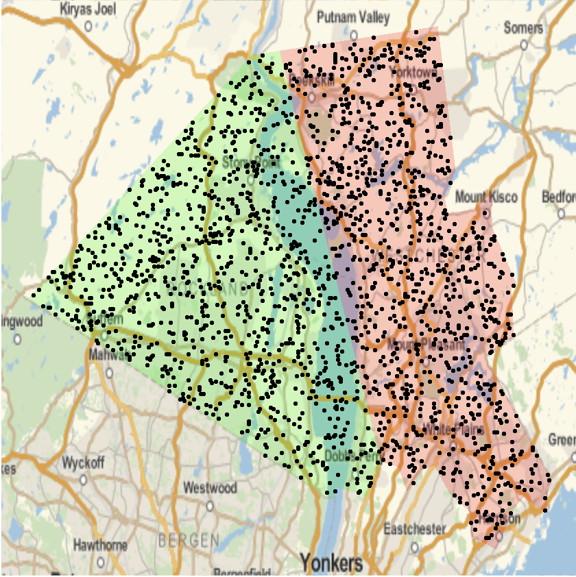
We can not iterate this by applying the districtSplit function to the two subregions:
out2state = districtSplit[outstate[[1]], outstate[[3]]];
out3state = districtSplit[outstate[[2]], outstate[[4]]];
Show[GeoGraphics[{Opacity[0.6], Red, out2state[[1]]}],
 GeoGraphics[{Opacity[0.6], Green, out2state[[2]]}],
 GeoGraphics[{Opacity[0.6], Yellow, out3state[[1]]}],
 GeoGraphics[{Opacity[0.6], Blue, out3state[[2]]}],
 GeoGraphics[Point /@ datateststate], AspectRatio -> 1]
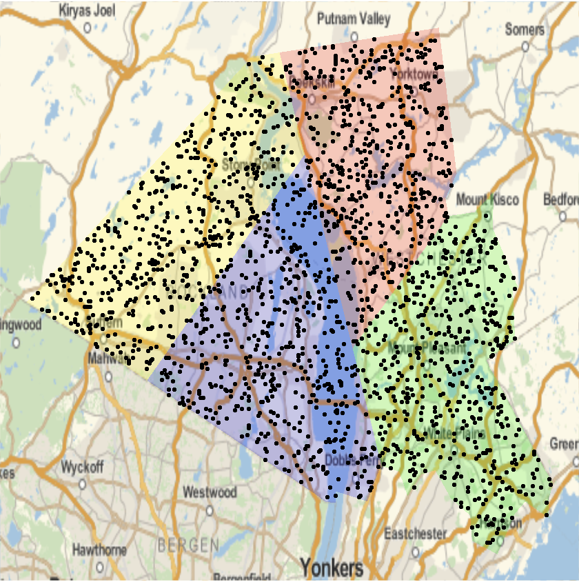
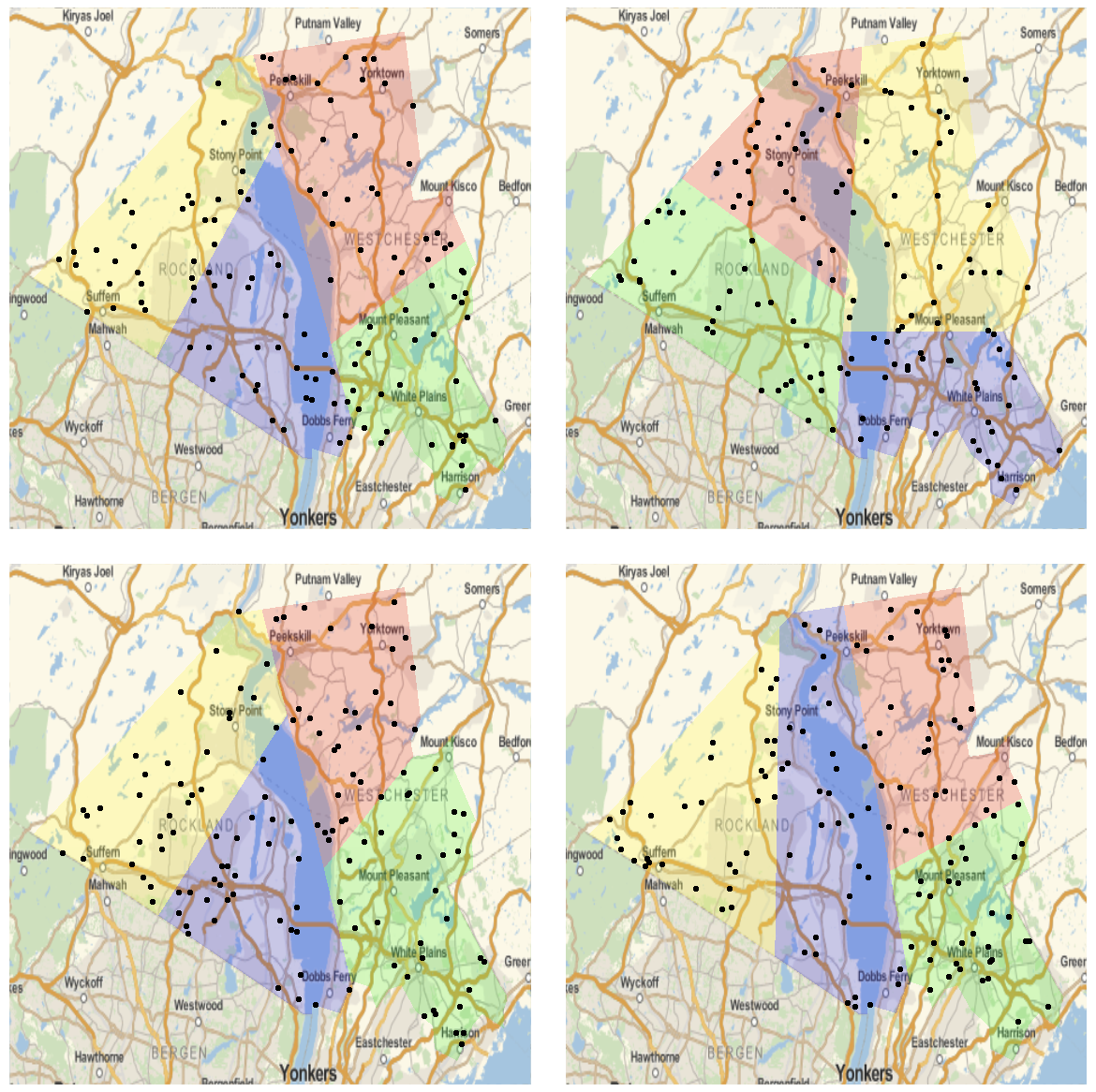
We can run the algorithm for fewer points and observe that each set of random points leads to slightly different splits (as expected).
Splitting for states
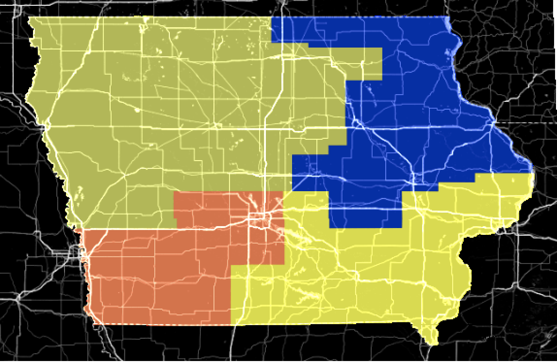
Next we can try to split states into districts. We start with Iowa. First we look at the actual voting districts in Iowa.
iowadistricts = Flatten[Position[polygoncodes, #] & /@ Select[polygoncodes, #[[1]] == "19" &]];

styling = {GeoBackground -> GeoStyling["StreetMapNoLabels", GeoStylingImageFunction -> (ImageAdjust@
ColorNegate@ColorConvert[#1, "Grayscale"] &)], GeoScaleBar -> Placed[{"Metric", "Imperial"}, {Right, Bottom}],
GeoRangePadding -> Full, ImageSize -> Large};

ImageAdd[GeoGraphics[Entity["AdministrativeDivision", {"Iowa", "UnitedStates"}], styling],
 GeoGraphics[Riffle[RandomColor[Length[iowadistricts]], districtsUS[[1, 2, 2]][[iowadistricts]]], GeoBackground -> None]]
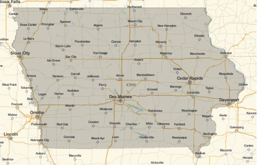
First we request the polygon for the state of Iowa.
polygonIowageo = Entity["AdministrativeDivision", {"Iowa", "UnitedStates"}]["Polygon"];
GeoGraphics[polygonIowageo]
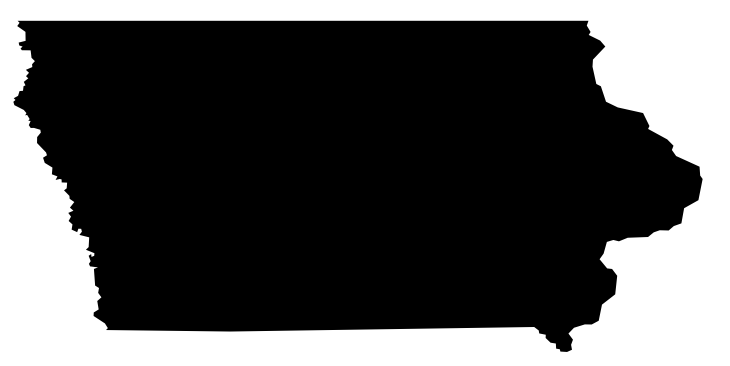
The (non-geo) polygon is then obtained by
polygonIowa = Polygon[Reverse /@ ((polygonIowageo /. {GeoPosition -> Identity, Polygon -> Identity}))[[1]]];
Graphics[polygonIowa]
We then "generate voters" at random positions.
votersIowa = RandomPoint[polygonIowa, 1000];
Now we can split the state into districts
out1Iowa = districtSplit[polygonIowa, votersIowa];
Then we split the resulting regions:
out2Iowa = districtSplit[out1Iowa[[1]], out1Iowa[[3]]];
out3Iowa = districtSplit[out1Iowa[[2]], out1Iowa[[4]]];
We can now plot the result
Show[GeoGraphics[{Opacity[0.6], Red, out2Iowa[[1]]}],
 GeoGraphics[{Opacity[0.6], Green, out2Iowa[[2]]}],
 GeoGraphics[{Opacity[0.6], Yellow, out3Iowa[[1]]}],
 GeoGraphics[{Opacity[0.6], Blue, out3Iowa[[2]]}],
 GeoGraphics[Point /@ votersIowa], AspectRatio -> 1/GoldenRatio]
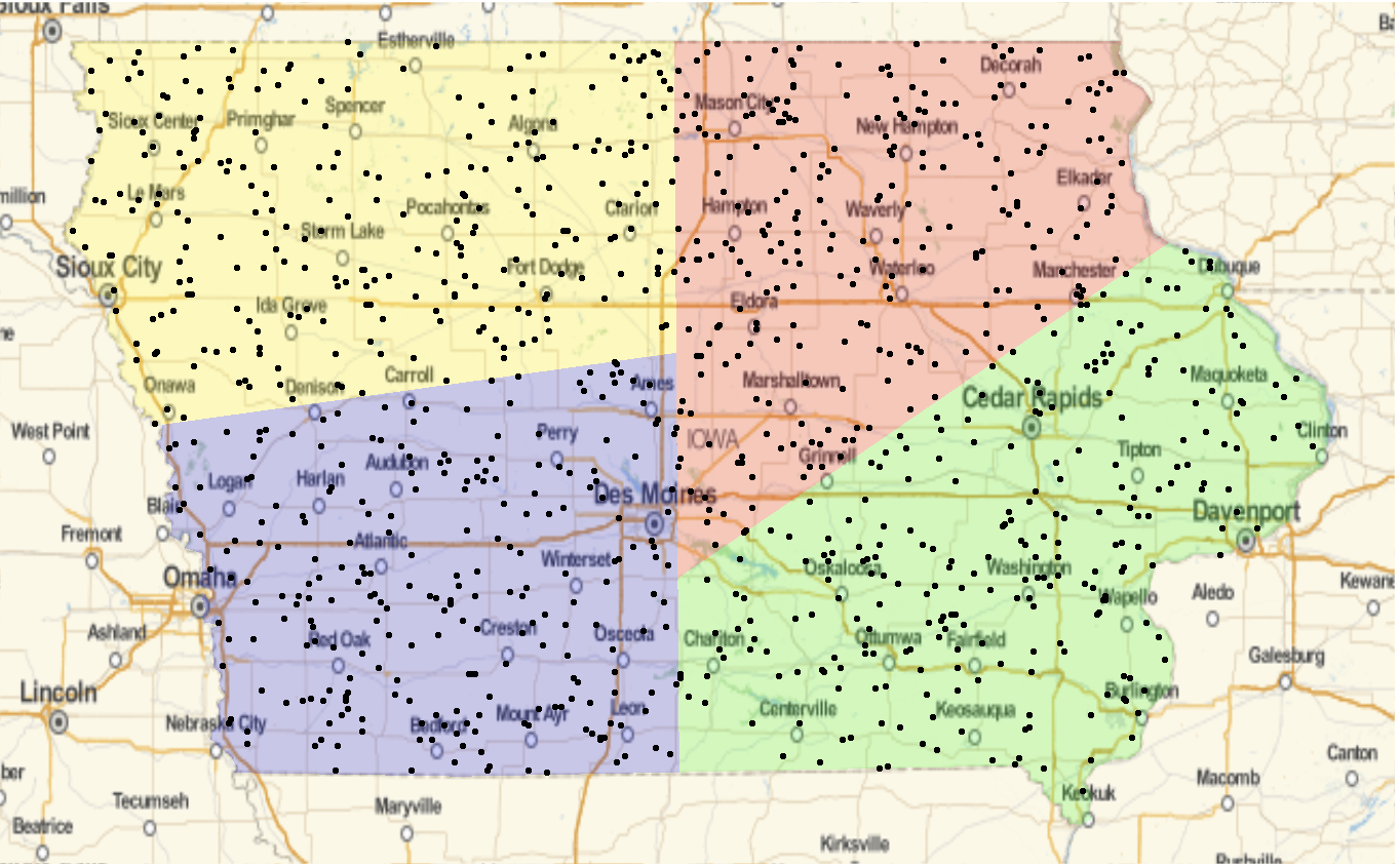
This of course assumes that the voters are "drawn" from a uniform spatial distribution.
More realistic population densities
Up to now the populations of voters have been assumed to be uniformly distributed in the region. To be more realistic we need very high resolution population density data, which can be obtained from this website: https://www2.census.gov/geo/tiger/TIGER2010BLKPOPHU/ I will be using a sampling approach and generate a distribution of voters drawn from the population census data.
Let's load and extract the data for Iowa (the 19 in the file name is the identifier of Iowa):
iowadata = Import["/Users/thiel/Desktop/tabblock2010_19_pophu/tabblock2010_19_pophu.shp", "Data"];
The file contains
iowadata[[1, 2, 2]] // Length
216007 polygonal subregions for Iowa; and
iowadata[[1, 4]][[2, 8]][[2]]
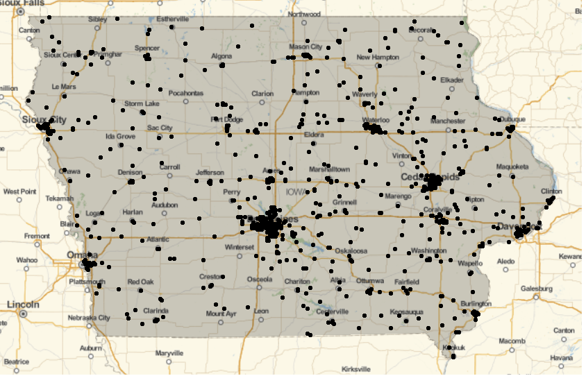
contains the 216007 corresponding entries of number of people living in these subregions. We choose 1000 regions at random (multiple choices of the same region are allowed), with weights corresponding to their respective population:
randomtexasregions = RandomChoice[iowadata[[1, 4]][[2, 8]][[2]] -> Range[Length[iowadata[[1, 2, 2, All]]]], 1000];
Then we choose the position of a person living in that region (and delete the failed attempts, e.g. when we have regions that have holes):
iowavotersample = Cases[RandomPoint[(iowadata[[1, 2, 2, #]] /. GeoPosition -> Identity)] & /@ randomtexasregions, {_, _}];
We can then plot the choice:
GeoGraphics[{Polygon[Entity["AdministrativeDivision", {"Iowa", "UnitedStates"}]], Point /@ GeoPosition /@ iowavotersample}]
Next, we use those points for the splitting algorithm (note that we have to invert the coordinates!).
out1Iowapop = districtSplit[polygonIowa, Reverse /@ iowavotersample];
out2Iowapop = districtSplit[out1Iowapop[[1]], out1Iowapop[[3]]];
out3Iowapop = districtSplit[out1Iowapop[[2]], out1Iowapop[[4]]];
We can then plot the resulting districting:
styling = {GeoBackground -> GeoStyling["StreetMapNoLabels", GeoStylingImageFunction -> (ImageAdjust@ColorConvert[0.98 #1, "Grayscale"] &)], GeoScaleBar -> Placed[{"Metric", "Imperial"}, {Right, Bottom}], GeoRangePadding -> Full, ImageSize -> Large};
Show[
GeoGraphics[Join[{Opacity[0.5], Red}, Point /@ (GeoPosition /@ iowavotersample)], styling],
GeoGraphics[{Opacity[1], Red, out2Iowapop[[1]]}, GeoBackground -> None],
GeoGraphics[{Opacity[1], Green, out2Iowapop[[2]]}, GeoBackground -> None],
GeoGraphics[{Opacity[1], Yellow, out3Iowapop[[1]]}, GeoBackground -> None],
GeoGraphics[{Opacity[1], Blue, out3Iowapop[[2]]}, GeoBackground -> None], ImageSize -> Full]
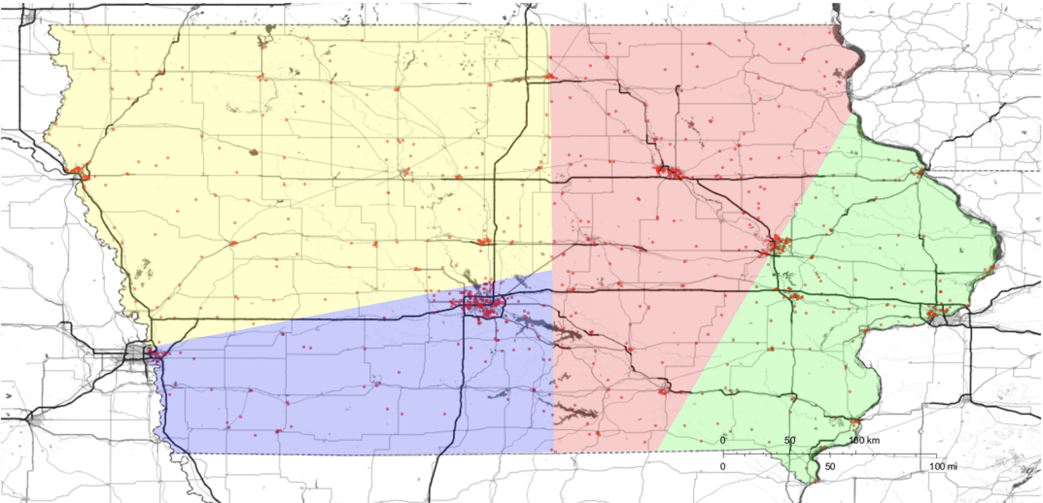
The results can be improved by using more voters. The split is much better and takes the population distribution into consideration. But the partitioning cuts through population centres (cities) which divides communities.
Splitting into other than 2^n districts
Up do now we can only half the regions, and therefore obtain splits into 2^n regions. This can easily be fixed in the definitions of the functions. First we again define the Utility functions:
ClearAll["Global`*"]
(*Utility functions*)

boundingcirclef[data_] := List @@ BoundingRegion[data, "MinDisk"]

pointsonpluscircle[p_] := 1.1 boundingcircle[[2]] {Cos[p], Sin[p]}

radiusperpendicular[p_] := RotationMatrix[Pi/2].{Cos[p], Sin[p]}

lengthprojection[p_, datain_] := If[EvenQ[Length[datain]], Median[radiusperpendicular[p].(# - boundingcircle[[1]]) & /@ datain],
Mean[{Median[#], Nearest[Complement[#, {Median[#]}], Median[#]][[1]]}] &@(radiusperpendicular[p].(# - boundingcircle[[1]]) & /@ datain)]

lengthprojectionnthpart[p_, datain_, m_] := Mean[Sort[#][[{Floor[Length[#]/m], Floor[Length[#]/m] + 1}]]] &@(radiusperpendicular[p].(# - boundingcircle[[1]]) & /@ datain)

linesplitlong[theta_, datain_] := {# + 3000*boundingcirclef[datain][[2]]*pointsonpluscircle[theta], # - 3000*boundingcirclef[datain][[2]]* pointsonpluscircle[theta]} &@(pointsonpluscircle[theta] + boundingcircle[[1]] + lengthprojection[theta, datain]*radiusperpendicular[theta])

linesplitlongnthpart[theta_, datain_, m_] := {# + 3000*boundingcirclef[datain][[2]]*pointsonpluscircle[theta], # - 3000*boundingcirclef[datain][[2]]*
pointsonpluscircle[theta]} &@(pointsonpluscircle[theta] + boundingcircle[[1]] + lengthprojectionnthpart[theta, datain, m]*radiusperpendicular[theta])

region1[point1_, point2_, regionin_] := ImplicitRegion[{x, y} \[Element] regionin && y >= point2[[2]] + (point2[[2]] - point1[[2]])/(point2[[1]] - point1[[1]]) (x - point2[[1]]), {x, y}]

region2[point1_, point2_, regionin_] := ImplicitRegion[{x, y} \[Element] regionin && y < point2[[2]] + (point2[[2]] - point1[[2]])/(point2[[1]] - point1[[1]]) (x - point2[[1]]), {x, y}]

implicitRegion2polygon[impregion_] := Module[{},
Polygon[Part[MeshCoordinates[#], DeleteDuplicates@Level[MeshCells[#, 1], {-1}]]] &@DiscretizeGraphics[Graphics[((RegionPlot[Evaluate[#[[1, 2]]], {x, y} \[Element] #[[1, 1, 2]]] /. Polygon[___] -> Nothing) /. Graphics -> List)[[1]]]] & @impregion]
Then we define the districting functions:
districtSplit[regionin_, datain_] := Module[{},
boundingcirclesplitline = boundingcirclef[datain];
boundingcircle = boundingcirclef[datain];
splitline = Line[{MeshCoordinates[MinimalBy[Table[{theta, RegionIntersection[BoundaryDiscretizeRegion @regionin, #] &@
Line[linesplitlong[theta, datain]]}, {theta, 0, 2 Pi, 0.01}], ArcLength[#[[2]]] &][[1, 2]]][[{1, -1}]]}];
(*Print[splitline];*)
{implicitRegion2polygon[region1[#[[1]], #[[2]], #[[3]]] &@Flatten[Append[splitline[[1]], regionin], 1]],
 implicitRegion2polygon[region2[#[[1]], #[[2]], #[[3]]] &@Flatten[Append[splitline[[1]], regionin], 1]],
 Select[datain, RegionMember[region1[#[[1]], #[[2]], #[[3]]] &@Flatten[Append[splitline[[1]], regionin], 1], #] &],
 Select[datain, RegionMember[region2[#[[1]], #[[2]], #[[3]]] &@Flatten[Append[splitline[[1]], regionin], 1], #] &]}]
and another function for "non-halving-districting":
districtSplitnthpart[regionin_, datain_, m_] := Module[{},
boundingcirclesplitline = boundingcirclef[datain];
boundingcircle = boundingcirclef[datain];
splitline = Line[{MeshCoordinates[MinimalBy[Table[{theta, RegionIntersection[BoundaryDiscretizeRegion @regionin, #] &@
Line[linesplitlongnthpart[theta, datain, m]]}, {theta, 0, 2 Pi, 0.01}], ArcLength[#[[2]]] &][[1, 2]]][[{1, -1}]]}];
(*Print[splitline];*)
{implicitRegion2polygon[region1[#[[1]], #[[2]], #[[3]]] &@Flatten[Append[splitline[[1]], regionin], 1]],
 implicitRegion2polygon[region2[#[[1]], #[[2]], #[[3]]] &@Flatten[Append[splitline[[1]], regionin], 1]],
Select[datain, RegionMember[region1[#[[1]], #[[2]], #[[3]]] &@Flatten[Append[splitline[[1]], regionin], 1], #] &],
Select[datain, RegionMember[region2[#[[1]], #[[2]], #[[3]]] &@Flatten[Append[splitline[[1]], regionin], 1], #] &]}]
Now we can first split off one third of the voters.
outtriple1 = districtSplitnthpart[polygonIowa, votersIowa, 3];
The second part of the output needs to be split into 2 subregions. That will give three regions of (nearly) equal number of voters.
outtriple2 = districtSplit[outtriple1[[2]], outtriple1[[4]]];
We can plot this like so
Show[GeoGraphics[{Opacity[0.6], Red, outtriple1[[1]]}],
 GeoGraphics[{Opacity[0.6], Green, outtriple2[[1]]}],
 GeoGraphics[{Opacity[0.6], Yellow, outtriple2[[2]]}],
 GeoGraphics[Point /@ votersIowa], AspectRatio -> 1/GoldenRatio]
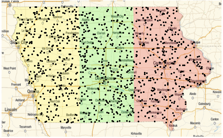
With these functions we can now split into any number of voting districts.
We can now run this for all states
We will show the results of this slightly longer simulation at a later point in time.
Indications for Gerrymandering in actual electoral districts
For this part of the analysis we will use the electoral districts as used above:
SetDirectory[NotebookDirectory[]];
districtsUS = Import["cb_2016_us_cd115_5m/cb_2016_us_cd115_5m.shp", "Data"];
polygoncodes = StringPartition[#, 2] & /@ (districtsUS[[1, -2 ;;, 2, 4]][[2, 2]]);
stateCodes = Join[#[[2]] -> #[[3]] & /@ SortBy[Partition[Flatten[Import["https://www.mcc.co.mercer.pa.us/dps/state_fips_code_listing.htm", "Data"][[1, 2 ;;]]], 3], #[[2]] &], {"69" -> "Northern Marianna Islands"}]

As mentioned above there are
Length[districtsUS[[1, 2, 2]]]
411 electoral districts. We can plot the districts
GeoGraphics[districtsUS[[1, 2, 2]][[1]]]
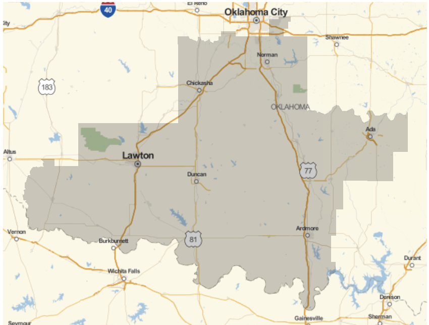
and perform analyses on them. For example we can calculate its area:
GeoArea[districtsUS[[1, 2, 2]][[1]]]
(*Quantity[9934.76, ("Miles")^2]*)
We can also plot the boundary
Graphics[Line[Reverse /@ (districtsUS[[1, 2, 2]][[1, 1, 1]])]]
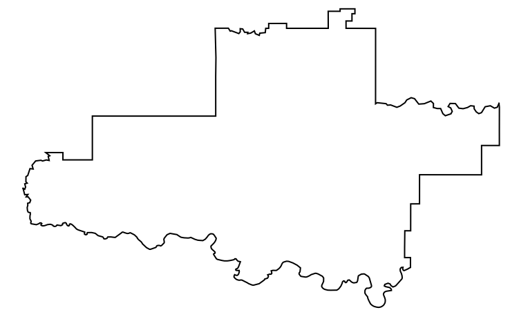
And calculate the perimeter length
ArcLength[#] & @Line[districtsUS[[1, 2, 2]][[1, 1, 1]]]
(*10.7136*)
A more interesting measure is the ratio of area to circumference:
RegionMeasure[Region[#]]/RegionMeasure[RegionBoundary[Region[#]]] &@Polygon[districtsUS[[1, 2, 2]][[1, 1, 1]]]
(*0.235957*)
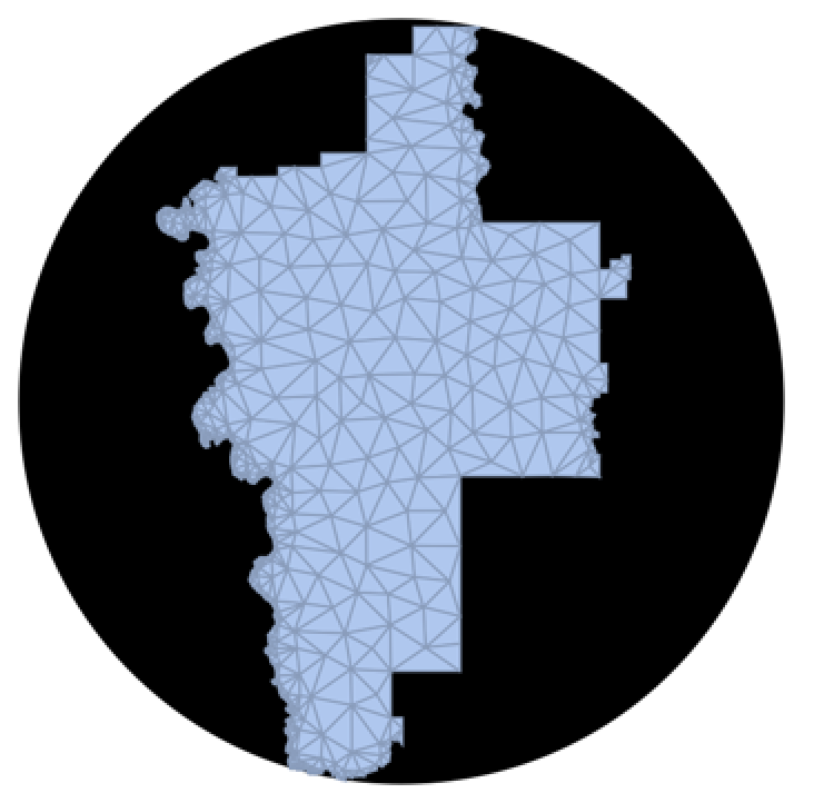
For a circle that would be 1/2, which is the largest number that this ratio can have for any region; the more elongated the area and the wigglier the boundary the smaller this ratio will be. Another important measure is given by the ratio of the areas of the district and the area of the circumscribed disk.
Show[Graphics[BoundingRegion[#, "MinDisk"]], #] &@DiscretizeRegion[Polygon[districtsUS[[1, 2, 2]][[1, 1, 1]]]]
(Area[#]/Area[BoundingRegion[#, "MinDisk"]]) &@DiscretizeRegion[Polygon[districtsUS[[1, 2, 2]][[1, 1, 1]]]]
(*0.38916*)
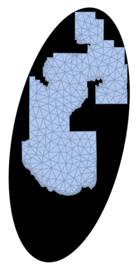
One could use different circumscribed objects like an ellipse:
Show[Graphics[BoundingRegion[#, "FastEllipse"]], #] &@DiscretizeRegion[Polygon[districtsUS[[1, 2, 2]][[2, 1, 1]]]]
This is the ratio of the areas:
(Area[#]/Area[BoundingRegion[#, "FastEllipse"]]) &@DiscretizeRegion[Polygon[districtsUS[[1, 2, 2]][[2, 1, 1]]]]
(*0.460971*)
Further measures can be found on the website: "https://www.scientificamerican.com/article/the-mathematicians-who-want-to-save-democracy/"
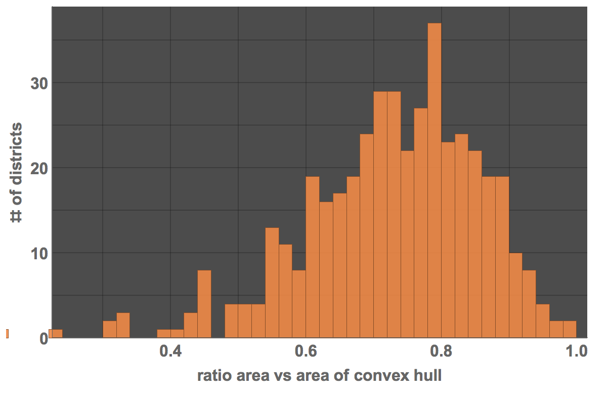
i) the ratio of the area of the district to the area of its convex hull
Area[#]/Area[ConvexHullMesh[(# /. Polygon -> List)[[1]]]] &@Polygon[districtsUS[[1, 2, 2]][[2, 1, 1]]]
(*0.739074*)
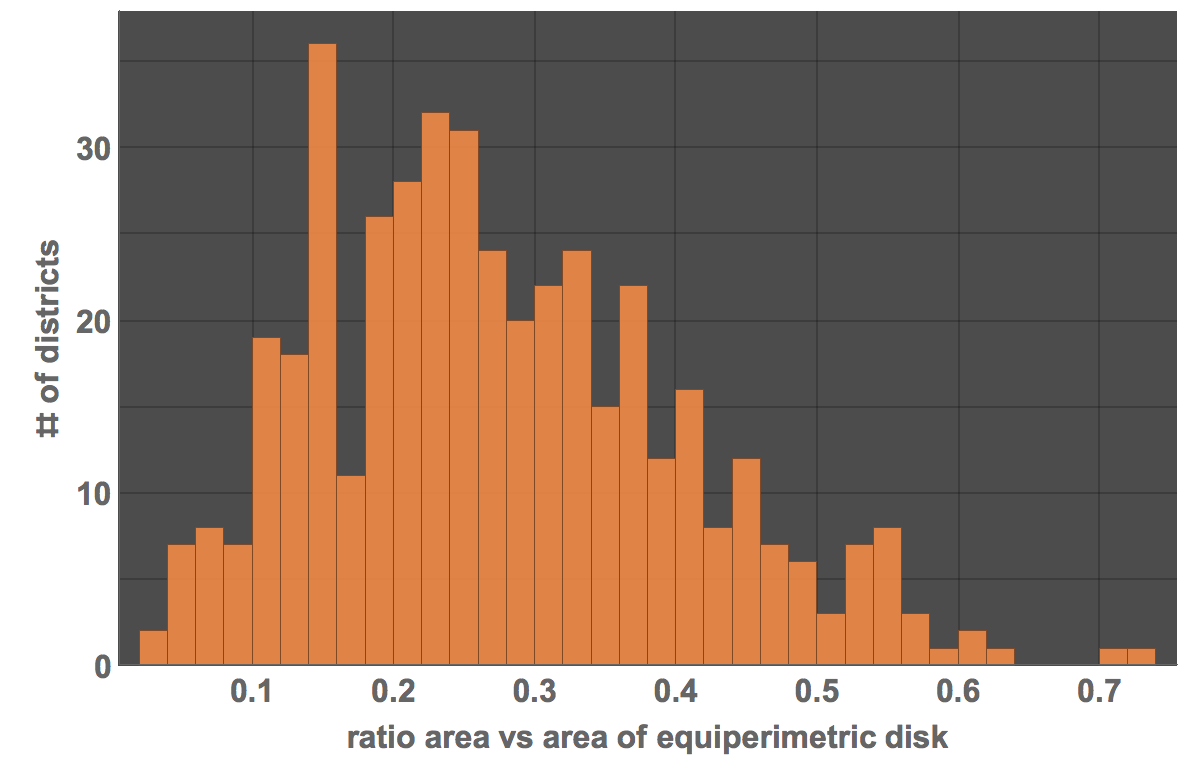
ii) the ratio of the area of the district as compared to the area of a circle with the same parameter:
Area[#]/(Pi (Perimeter[#]/(2 Pi))^2) &@Polygon[districtsUS[[1, 2, 2]][[2, 1, 1]]]
(*0.23955*)
Next we should try to run these measures on a set of districts:
GraphicsGrid[{GeoGraphics /@ districtsUS[[1, 2, 2]][[1 ;; 3]],
Show[Graphics[BoundingRegion[#, "MinDisk"]], #] & /@ Table[DiscretizeRegion[Polygon[Reverse /@ districtsUS[[1, 2, 2]][[k, 1, 1]]]], {k, 1, 3}]}, ImageSize -> Large]
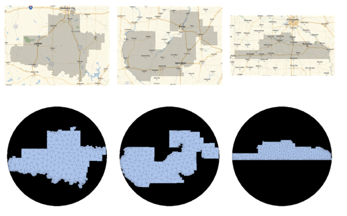
Let's first calculate the ratio of district area to circumscribed disk for all districts:
areatoCircleratio =
  Table[(Area[#]/Area[BoundingRegion[#, "MinDisk"]]) &@(RegionUnion @@
   DiscretizeRegion /@ (If[Head[#] === Polygon, #, filledCurveRegion[[1]]] & /@
   Flatten[{districtsUS[[1, 2, 2]][[k]]}] /. GeoPosition -> Identity)), {k, 1, Length[districtsUS[[1, 2, 2]]]}];
We can not represent these values in a histogram
Histogram[areatoCircleratio, 30, PlotTheme -> "Marketing",
 FrameLabel -> {"ratio area vs area of circumscribe circle", "# of districts"}, LabelStyle -> Directive[Bold, 16]]
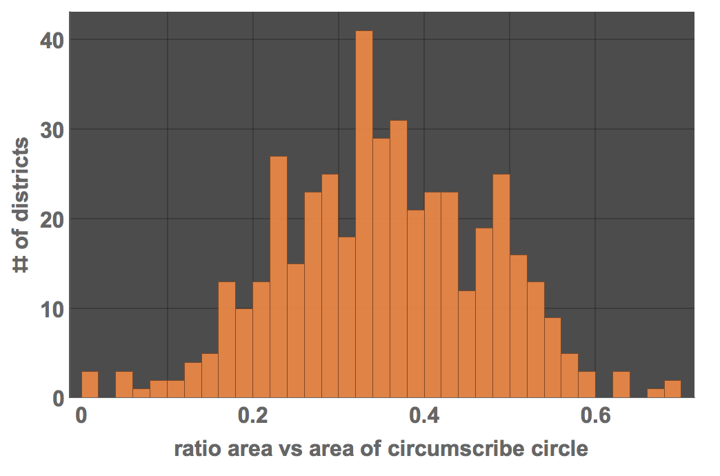
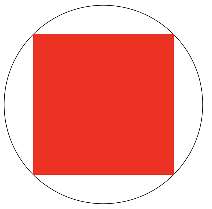
In particular the small values indicate highly elongated districts. A rectangular region
Graphics[{Circle[{0, 0}, Sqrt[2]], Red, Rectangle[{-1, -1}, {1, 1}]}]
would have a ratio of
Area[Rectangle[{-1, -1}, {1, 1}]]/Area[Disk[{0, 0}, Sqrt[2]]] // N
(*0.63662*)
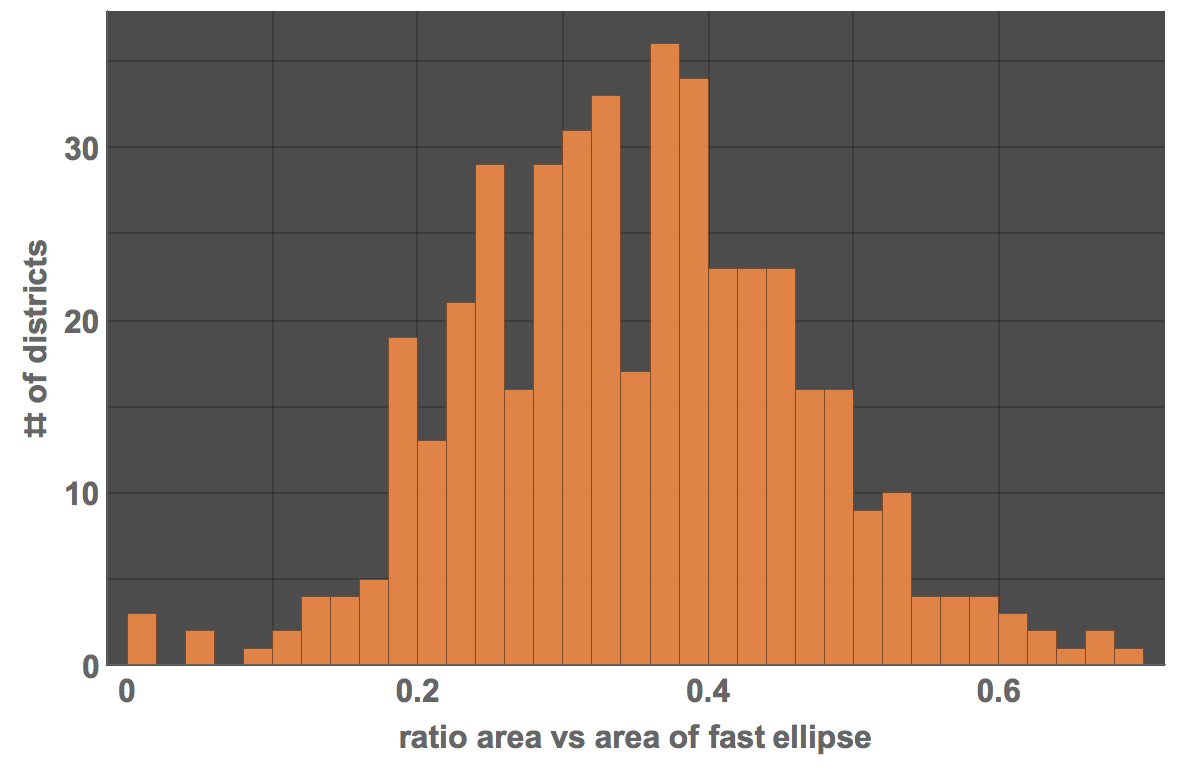
Next, we calculate the ratio for the fast ellipse:
areatoEllipseratio =
  Table[(Area[#]/Area[BoundingRegion[#, "FastEllipse"]]) &@(RegionUnion @@
  DiscretizeRegion /@ (If[Head[#] === Polygon, #, filledCurveRegion[[1]]] & /@
  Flatten[{districtsUS[[1, 2, 2]][[k]]}] /. GeoPosition -> Identity)), {k, 1, Length[districtsUS[[1, 2, 2]]]}];
This gives the histogram:
Histogram[areatoEllipseratio, 30, PlotTheme -> "Marketing", FrameLabel -> {"ratio area vs area of fast ellipse", "# of districts"}, LabelStyle -> Directive[Bold, 16], ImageSize -> Large]
Next up are the area ratios wrt the convex hull:
areatoConvexHullratio =
  Table[Area[#]/Area[ConvexHullMesh[RandomPoint[RegionBoundary[#], 100]]] &@(RegionUnion @@
  DiscretizeRegion /@ (If[Head[#] === Polygon, #, filledCurveRegion[[1]]] & /@
  Flatten[{districtsUS[[1, 2, 2]][[k]]}] /. GeoPosition -> Identity)), {k, 1, Length[districtsUS[[1, 2, 2]]]}];

Histogram[areatoConvexHullratio, 30, PlotTheme -> "Marketing",
 FrameLabel -> {"ratio area vs area of convex hull",
   "# of districts"}, LabelStyle -> Directive[Bold, 16],
 ImageSize -> Large]
The ratio of areas of district and equi-perimetric disk are
arearatioequivalentDisk =
Table[Area[#]/(Pi (Perimeter[#]/(2 Pi))^2) &@(RegionUnion @@
DiscretizeRegion /@ (If[Head[#] === Polygon, #, filledCurveRegion[[1]]] & /@
Flatten[{districtsUS[[1, 2, 2]][[k]]}] /. GeoPosition -> Identity)), {k, 1, Length[districtsUS[[1, 2, 2]]]}];

Histogram[arearatioequivalentDisk, 30, PlotTheme -> "Marketing", FrameLabel -> {"ratio area vs area of equiperimetric disk", "# of districts"}, LabelStyle -> Directive[Bold, 16], ImageSize -> Large]
Last but not least we generate random points in the districts and then connect each of the with a straight line. We then compute the percentage of lines that are completely within the district. This is a measure of convexity - and takes a while to compute.
Monitor[convexitymeasure =
  Table[N[Count[#, False]/Length[#]] & @(MemberQ[#, False] & /@ (RegionMember[(RegionUnion @@
  DiscretizeRegion /@ (If[Head[#] === Polygon, #, filledCurveRegion[[1]]] & /@
  Flatten[{districtsUS[[1, 2, 2]][[k]]}] /. GeoPosition -> Identity))] /@
  RandomPoint[#, 100] & /@ (Line /@ Flatten[Outer[List, #, #, 1] & @(RandomPoint[(RegionUnion @@
  DiscretizeRegion /@ (If[Head[#] === Polygon, #, filledCurveRegion[[1]]] & /@
  Flatten[{districtsUS[[1, 2, 2]][[k]]}] /. GeoPosition -> Identity)), 40])*UpperTriangularize[ConstantArray[1, {40, 40}], 1] /. {{0.`, 0.`}, {0.`, 0.`}} -> Nothing, 1]))), {k, 1,Length[districtsUS[[1, 2, 2]]]}], k]
The closer the values to unity, the "more convex" is the shape:
ListPlot[convexitymeasure, PlotTheme -> "Marketing", FrameLabel -> {"district number", "convexity meaure"}, LabelStyle -> Directive[Bold, 16]]
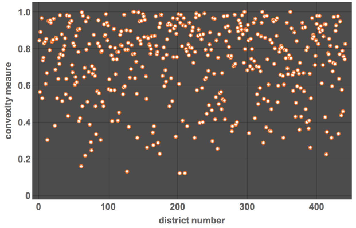
We can for example choose the districts with the lowest values:
leastconvex = Flatten[Position[convexitymeasure, #] & /@ Sort[convexitymeasure][[1 ;; 5]]]
(*{203, 210, 127, 61, 67}*)
Visual inspection of the respective districts:
GraphicsRow[(GeoGraphics@districtsUS[[1, 2, 2]][[#]]) & /@ leastconvex]

shows that they are very much meandering.
Statistical comparison of districts based on the measures
This will be shown at a later point in time. We have developed a number of measures and extremes of these measures suggest Gerrymandering issues. A more thorough analysis is required which is beyond the scope of this particular post.
Formation of areas of consensus
To be completed. This contains a simple model for voting patterns. It is based on the ISING model from statistical Physics. I will try to show how to calculate boundaries that benefit a given party. Assume we have a lattice of voters (later we will use graphs). I will explain the model; basically every box is a voter. A voter potentially changes their opinion when talking to its neighbours.
S = 50; subborn = 0.2;
world = RandomInteger[{0, 1}, {S, S}];
jump := RandomChoice[{{-1, 0}, {1, 0}, {0, -1}, {0, 1}}];
results = {world}; For[i = 2, i < 400, i++,
world = Table[RandomChoice[{subborn, 1 - subborn} -> {world[[i, j]], world[[i + jump[[1]] /. {Evaluate[S + 1] -> 1, Evaluate[0 -> S]},  j + jump[[2]] /. {Evaluate[S + 1] -> 1, Evaluate[0 -> S]}]]}], {i, 1, S}, {j, 1, S}];
 AppendTo[results, world];]
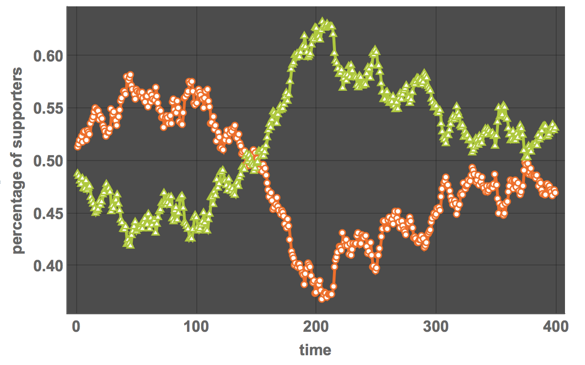
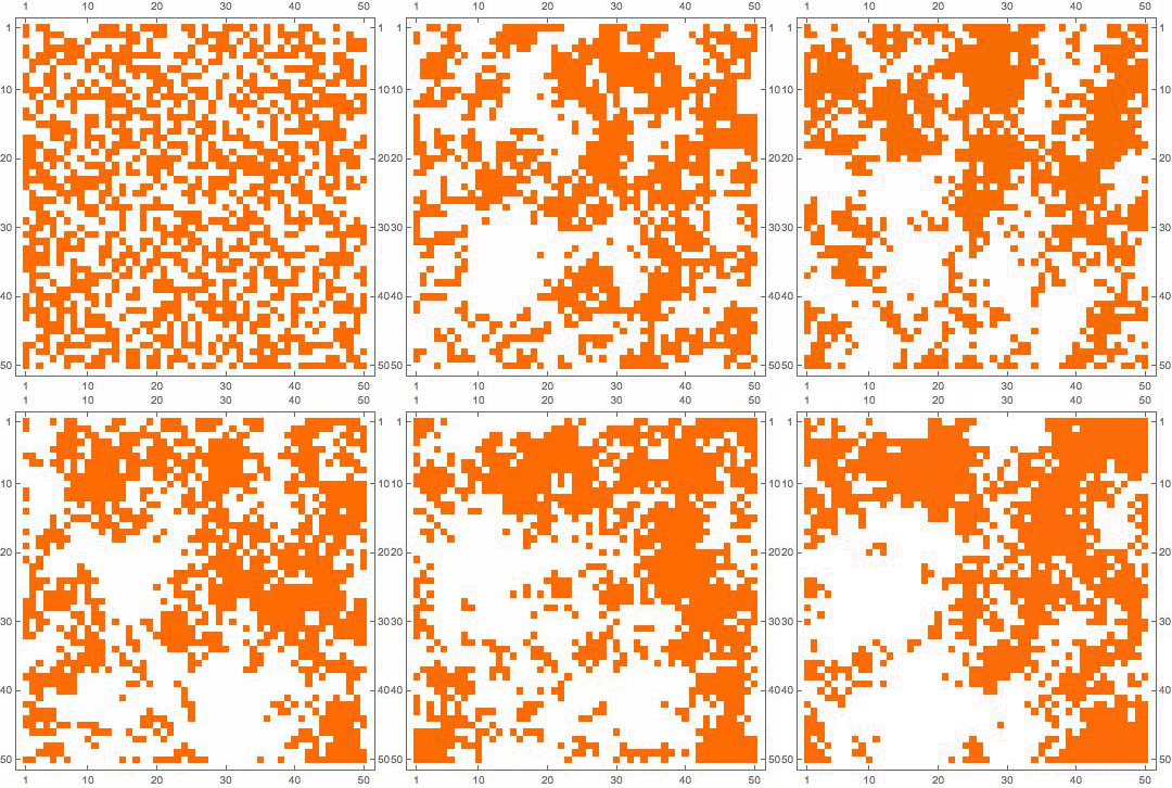
The variable "world" represents each voter at a lattice position. In every step this voter "speaks" to his/her neighbours and randomly adjusts their opinion to that person; there is also a stubborn-ess factor which models the propensity of a person not to change their opinion. Patches of similar opinions form spontaneously. We can first look at the percentages of people that support either choice.
ListLinePlot[{N[Count[Flatten[#], 0]/(S^2)] & /@ results, N[Count[Flatten[#], 1]/(S^2)] & /@ results},
PlotTheme -> "Marketing", ImageSize -> Large, FrameLabel -> {"time", "percentage of supporters"}, LabelStyle -> Directive[Bold, 16]]
Here is a video of the process:
Do[Export["~/Desktop/VoterVideo/frame" <> ToString[1000 + i] <> ".jpg", MatrixPlot[results[[i]]]], {i, 1, Length[results]}]
(*and then in terminal    convert -delay 25 -loop 0 frame*.jpg animated.gif *)
This can be used to compute areas to maximise the benefits of a choice of boundaries of voting districts for a given party. Let's look at the final situation:
MatrixPlot[results[[-1]]]
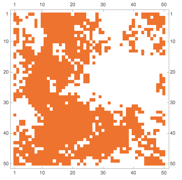
It is easy to see that at this point the opinion "one" is leading:
N[Count[Flatten[results[[-1]]], 1]/S^2]
(*0.5308*)

N[Count[Flatten[results[[-1]]], 0]/S^2]
(*0.4692*)
So there are 53 % in favour of "one" and 47% in favour of "zero". Let us first calculate the connected components:
connectedvoters = MorphologicalComponents[world, CornerNeighbors -> False];
MatrixPlot[connectedvoters]
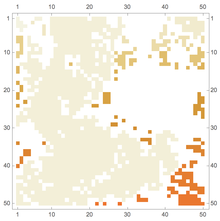
Let's look for the largest components:
Reverse@SortBy[Tally[Flatten[connectedvoters]], Last]

The largest cluster is made out of "0". We are interested in the "3"-cluster, which corresponds to many connected "ones".
Position[connectedvoters, 3] // Length
(*1081*)
We want to split the region into three districts of equal size. We therefore cannot put all of these points into one district. Let's only put 1/3 of all points in this cluster into a district. We will deal with that issue later. First we want to delete small components. In order to achieve this we convert the matrix to an image:
Image[Normal[SparseArray[Position[connectedvoters, 3] -> 1, {S, S}]]]
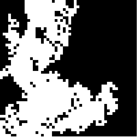
Let's calculate the connected components and delete small components:
imgint = DeleteSmallComponents[
  ColorNegate[
   MorphologicalComponents[
     Image[Normal[
       SparseArray[Position[connectedvoters, 3] -> 1, {S, S}]]],
     CornerNeighbors -> False] // Image], 55]
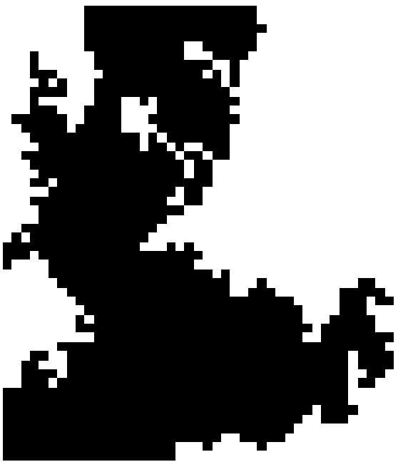
Let's choose the positions such that one district wins by a large margin. This district gets the points from this cluster - but only up to a third of all S^2 points:
district1 = Position[ImageData[imgint], 0.][[-Round[S^2/3] ;;]];
This district looks like this:
MatrixPlot[Normal[SparseArray[Position[ImageData[imgint], 0.][[-Round[S^2/3] ;;]] -> 1, {S, S}]]]
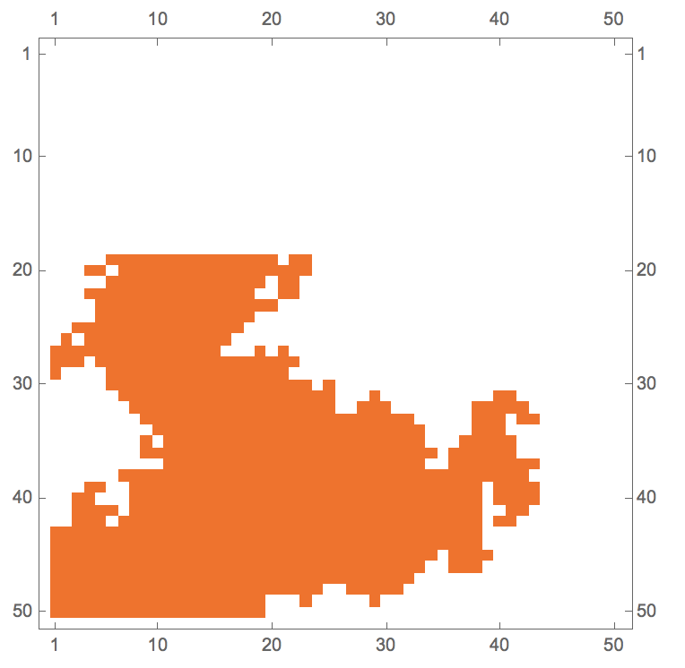
In this region there are over proportionally many white points. It clearly "meanders". The remaining points will be equally split into two other districts. The remaining points to distribute are:
remainingoints = Complement[Flatten[Table[{i, j}, {i, 1, S}, {j, 1, S}], 1], district1];
Let's calculate the ones with the largest distance wrt the Hamming distance:
maxdistpoints =
  Position[remainingoints, Max[Flatten[#]]] &@ DistanceMatrix[remainingoints, DistanceFunction -> ChessboardDistance];
We can determine the most frequent one:
mostfrequent = (Reverse@SortBy[Tally[Flatten[maxdistpoints]], Last])[[1, 1]]
(*2*)
This point is furthest away from most:
remainingoints[[mostfrequent]]
(*{1,2}*)
We now need to choose the nearest half of the remaining points to split the area into three (nearly) equal districts:
district2 = Nearest[remainingoints, remainingoints[[mostfrequent]], Round[S^2/3.], DistanceFunction -> ChessboardDistance];
The remaining points form district 3:
district3 = Complement[remainingoints, district2];
Let's plot the three regions:
MatrixPlot[Normal[SparseArray[Join[# -> 1 & /@ district1, # -> 2 & /@ district2, # -> 3 & /@ district3], {S, S}]]]
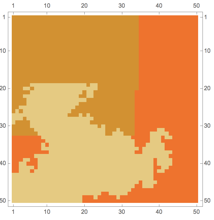
Let's finally see how the districts would vote - remember that most voters back opinion "one". In district one there are
N[Count[results[[-1]][[#[[1]], #[[2]]]] & /@ district1, 1]/Length[district1]]
93.5% of voters who back opinion "one". In district two there are
N[Count[results[[-1]][[#[[1]], #[[2]]]] & /@ district2, 1]/Length[district2]]
44.2% of voters who back opinion "one", so the majority backs "two". Finally, in region 3 there are
N[Count[results[[-1]][[#[[1]], #[[2]]]] & /@ district3, 1]/Length[district3]]
21.6% of voters who back "one", so the majority backs "two". Overall, two districts back opinion "two" and only one backs opinion "two". This reverts the result from the direct majority. Note that the regions have a (practically) equal number of voters.
Consensus time
On a separate note, we can also use this model (or similar models on social networks/graphs) to estimate consensus times:
Monitor[tab =
   Table[S = 10; subborn = 0.2; world = RandomInteger[{0, 1}, {S, S}];
     jump := RandomChoice[{{-1, 0}, {1, 0}, {0, -1}, {0, 1}}];
    var = Variance[Flatten[world]] // N; i = 0;
    While[var > 0,
     world = Table[
       RandomChoice[{subborn, 1 - subborn} -> {world[[i, j]],
          world[[i + jump[[1]] /. {Evaluate[S + 1] -> 1,
             Evaluate[0 -> S]},
           j + jump[[2]] /. {Evaluate[S + 1] -> 1,
             Evaluate[0 -> S]}]]}], {i, 1, S}, {j, 1, S}]; i++;
     var = Variance[Flatten[world]] // N;]; i, {k, 1, 1000}], k];
and the resulting histogram
Show[Histogram[tab, 70, "PDF"], Plot[Evaluate@PDF[Quiet@FindDistribution[tab], x], {x, 0, 1300}, PlotRange -> All, PlotStyle -> Red]]
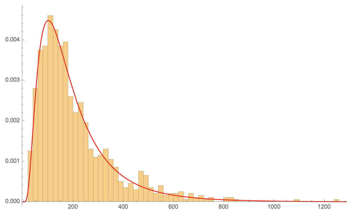
We observe that in some cases it takes very long to reach consensus. This has implications for the choice of the electoral period and therefore for the question whether the public opinion has settled down when an election takes place.
Conclusion
We have seen that there are ways of "fairly" splitting areas into electoral districts and that likewise one can choose boundaries such that one alternative benefits from that choice. In spite of the same ballots we can therefore obtain different outcomes of the elections, i.e. social choices. We have also calculated a number of measures to identify potential cases of Gerrymandering. We will post a more detailed analysis at a later point in time.
 Attachments: