Hi,
there are different ways of writing this. Here is an intuitive one (but not the most elegant):
(*Assuming the noise is independent for the processes*)
cW[\[Rho]_] := ItoProcess[{{0, 0}, IdentityMatrix[2]}, {{w1, w2}, {0, 0}}, t, {{1, \[Rho]}, {\[Rho], 1}}];
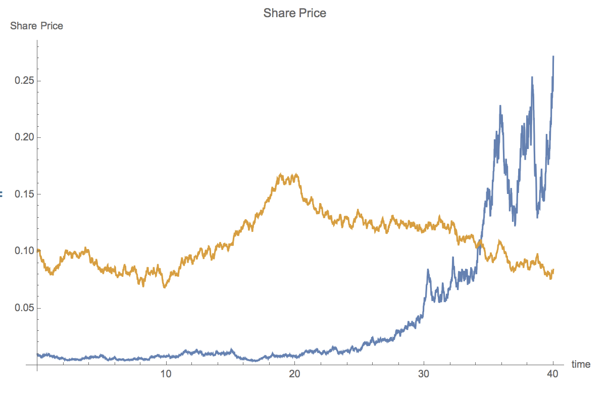
procGBMnoiseM = ItoProcess[{\[DifferentialD]S[t] == \[Mu][t] S[t] \[DifferentialD]t + \[Sigma] S[t] \[DifferentialD]Subscript[w, s][t], \[DifferentialD]\[Mu][t] == \[Lambda]*\[Mu][t]*(\[Mu]base - \[Mu][t]) \[DifferentialD]t + \[Sigma]2*\[DifferentialD]Subscript[w, r][t]}, {S[t], \[Mu][t]}, {{S, \[Mu]}, {0.01, \[Mu]base}},t, {Subscript[w, s], Subscript[w, r]} \[Distributed] cW[\[Rho]]];
This can be plotted like so:
ListLinePlot[RandomFunction[procGBMnoiseM /. { \[Sigma] -> 0.3, \[Sigma]2 -> 0.01, \[Lambda] -> 0.1, \[Mu]base -> 0.1, \[Rho] -> 0.0}, {0, 40, 0.01}], ImageSize -> Large, AxesLabel -> {"time", "Share Price"}, PlotLabel -> "Share Price"]
If you want more processes this can easily be generalised, of course. Here is a sort of "stochastic Kuramoto model", well sort of:
(*M is the number of trading partners, i.e. countries, \[Epsilon] is \
the strength of the interaction. The average trade is a number that \
describes the "normal/default trading volume of the country". *)
M = \
30; \[Epsilon] = 0.5; averagetrade =
 Table[RandomReal[{1, 5}], {i, 1, M}]; Do[
 Subscript[\[Omega], i] =
  RandomVariate[NormalDistribution[1., 0.025]], {i, 1, M}];
(*Obviously the adjacency matrix describes the trade network *)

adjacencymatrix = RandomChoice[{0.7, 0.3} -> {0, 1}, {M, M}];
(*The Ito process does not allow us to use variables with indices \
such as Subscript[x, i] ; this is why I generate strings for the \
variable names*)

variables = ToExpression @ Table["x" <> ToString[i], {i, 1, M}];
(*Here I generate the deterministic part of the equations. I assume a \
basic logistic dynamics (with the "carrying capacity" representing \
the averate trade value of the countries. I couple the countries \
diffusively similar to the Kuramoto system.*)

eqnsrhsdet =
  Table[Subscript[\[Omega],
    i] + \[Epsilon]/M Sum[
      adjacencymatrix[[j, i]]*(variables[[j]][t] -
         variables[[i]][t]), {j, 1, M}], {i, 1, M}];
(*This is \[Sigma] matrix of the noise. All noise terms are assumed \
to be independent. This is why this is a diagonal matrix. One could \
make the fluctuations of the trade of individual countries different \
by not using 0.3 everywhere on the diagonal.*)

eqnsrhsstoch = 0.4 IdentityMatrix[M];
(*Here we set initial conditions*)

initconds = Table[2 \[Pi] RandomReal[], {i, 1, M}] :
    (*\[Mu] quantifies how quick countries want to return to their \
default trading.*)
    proc =
   ItoProcess[{eqnsrhsdet, eqnsrhsstoch}, {variables, initconds}, {t,
     0}];
(*We generate the process. Time is from 0 to 10 and the sampling rate \
is 0.1*)
tseries = RandomFunction[proc, {0., 100., 0.1}, 1];
(*Just a wee plot*)
data = Mod[#, 2 \[Pi]] & /@
   Table[tseries["PathComponents"][[k]]["Paths"][[1, All, 2]], {k, 1,
     M}];
ListLinePlot[data[[1 ;; 4]], ImageSize -> Large]
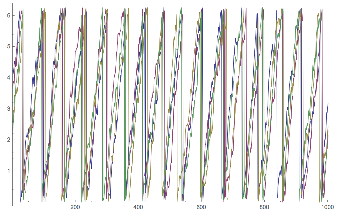
Please be aware that the comments refer to trade and different countries. This is quite a bit out of the context of where it was presented. So the model has a very (!) loose relationship (if at all) to trading. The trading example was rather used as an analogy to motivate the terms.
Cheers,
Marco


