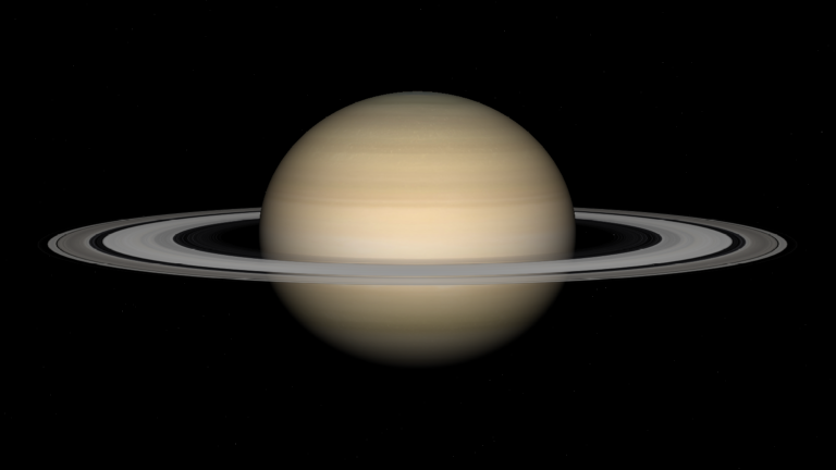
Creating a flyby simulation of a planetary scene in 3D involves multiple steps. This post walks you through the steps used to create the final animation (click this link or image below to play). I strongly recommend you watch the video in full screen mode with low lights so that all of the detail is visible. Some of it is subtle.
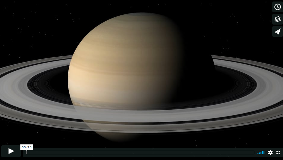
The Vimeo video hosting service has a habit of auto-advancing to the next video, but what it chooses as the next one is often strange in my opinion, so be prepared to click the back button to replay it.
Creating the Planet
Saturn can be treated as an oblate spheroid which we can model in the Wolfram Language using ParametricPlot3D and textures. EntityValue can give us a few pointers to get things scaled properly. First, we need to know the equatorial radius of the planet and its oblateness (e.g. how flattened it is at the poles compared to the equator).
saturnradius =
  QuantityMagnitude[Entity["Planet", "Saturn"]["EquatorialRadius"],
   "Kilometers"];

saturnoblateness = Entity["Planet", "Saturn"]["Oblateness"];

texture =
  ImageReflect[EntityValue[Entity["Planet", "Saturn"],
   "CylindricalEquidistantTexture"], Bottom];
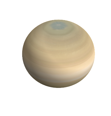
With the data above, we can construct a ParametericPlot3D of an oblate spheroid scaled to the dimensions of Saturn. We use the curated data from above to perform the scaling.
planet = ParametricPlot3D[{saturnradius Cos[t] Sin[p],
   saturnradius Sin[t] Sin[
     p], (1 - saturnoblateness) saturnradius Cos[p]}, {t, 0,
   2 Pi}, {p, 0, \[Pi]}, Mesh -> None, PlotStyle -> Texture[texture],
  Lighting -> "Neutral", Boxed -> False, Axes -> False,
  PlotPoints -> 100]
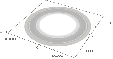
Creating the Rings
The rings of Saturn lie along a plane and can be modeled as an annulus with radial color and opacity variation. We make use of a texture obtained from https://www.classe.cornell.edu/~seb/celestia/hutchison/saturn-rings.png and stored as a CloudObject in the Wolfram Cloud and use ParametricPlot3D to apply this color and opacity texture to the annulus.
ringalpha = Import[
CloudObject[
   "https://www.wolframcloud.com/objects/4e39f856-1c09-44d1-b2a9-\
00ffd480b6dd"]];

ringinnerradius = 74510;

ringouterradius = 140390;

rings = ParametricPlot3D[{r Cos[t], r Sin[t], 0}, {r, ringinnerradius,
    ringouterradius}, {t, 0, 2 Pi}, Mesh -> None,
  PlotStyle -> Texture[ringalpha], PlotPoints -> 100]
Creating a Star Backdrop
To give some additional subtle detail, we can provide more sense of motion and context for the opacity variations in the rings by providing a backdrop of stars. We make use of EntityValue to obtain position and brightness data for stars visible to the naked-eye (nearly 9,000 stars). This takes a couple minutes depending on your network connection.
In[9]:= stardata =
  EntityValue[
   EntityClass["Star", "NakedEyeStar"], {"RightAscension", "Declination",
    "ApparentMagnitude"}];

In[10]:= stardata // Length

Out[10]= 8910
To make use of the previous data in a graphical setting, we need to convert the Quantity objects to numbers in radians and also rescale the apparent magnitude brightness values to GrayLevel values between 0 and 1. We round the values of apparent magnitude since we want to optimize the rendering to make use of multi-point primitives later. Takes about a minute to convert the data into the necessary format.
In[11]:= triples = With[{magrange = MinMax[stardata[[All, 3]]]},
   {-QuantityMagnitude[#[[1]], "Radians"],
      QuantityMagnitude[#[[2]], "Radians"],
      Rescale[Round[#[[3]]], magrange, {1, .1}]} & /@ stardata];
Next, we group the stars based on their rounded values.
In[12]:= gb = GatherBy[triples, #[[3]] &];
We construct the star background primitives by converting the right ascension and declination values into Cartesian spherical coordinates and place them far enough outside of the Saturn system, 8 ring radii, that they can serve as a spherical backdrop assuming our camera stays inside this distance. Each magnitude value gets a specific GrayLevel and set of points with a single Point head.
In[13]:= stars = With[{r = 8 ringouterradius},
     {GrayLevel[#[[1, 3]]],
      Point[{-r Cos[#[[1]]] Sin[#[[2]] + Pi/2],
          r Sin[#[[1]]] Sin[#[[2]] + Pi/2], -r Cos[#[[2]] +
             Pi/2]} & /@ #]}] & /@ gb;
We can then assemble the star backdrop and assign a specific PointSize to all stars, using GrayLevel, not size, to represent brightness variations.
In[14]:= starscene = Graphics3D[{PointSize[.004], stars}];
Defining the Flight Path
The flightpath is a simple straight line. Its starts "in front" of Saturn at 4 ring radii out, and always keeps the camera pointed at the planet. The position of the camera changes with time. We construct the path using Interpolation, one for each Cartesian coordinate. As time progresses, the y-coordinate extends out to the side of Saturn so we don't hit it. We also modify the z-coordinate to start above the ring plane and drop below it at the end.
xfun = Interpolation[{4 ringouterradius, 3 ringouterradius, 2 ringouterradius,
     ringouterradius, 0, -ringouterradius}];

yfun = Interpolation[{0, ringouterradius, 2 ringouterradius,
    3 ringouterradius, 4 ringouterradius, 4 ringouterradius}];

zfun = Interpolation[{4 saturnradius, 3 saturnradius, 2 saturnradius,
    1 saturnradius, 0, -1 saturnradius}];
Assembling the Scene and Generating Frames
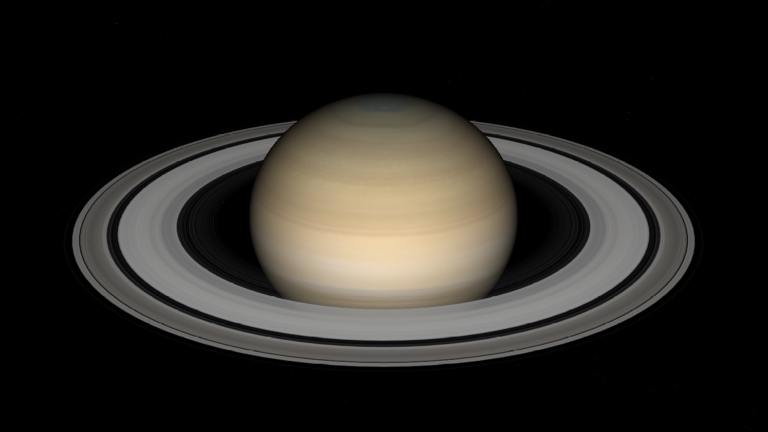
We can render an initial scene to get a sense of how it will look. We specify a point light source to look as if the system is being illuminated by the Sun from the "front".
gr = Show[{planet, Graphics3D[{Lighting -> {{"Ambient", GrayLevel[.33]}}, rings[[1]]}], starscene}, Background -> Black,
  ImageSize -> .4 {1920, 1080}, SphericalRegion -> True, ViewAngle -> Pi/10,
  ViewVector -> {{4 ringouterradius, 0, 1 saturnradius}, {0, 0, 0}},
  PlotRange -> All,
  Lighting -> {{"Ambient", GrayLevel[0]}, {"Point",
     White, {3 ringouterradius, 0, 3 saturnradius}}}]
The first step in animating the scene is to generate a list of frames. The elements are all static, but the camera position changes in time using ViewVector and making use of the interpolating functions created earlier. The time step is small so that we can obtain enough frames (600) to make the animation play back smoothly. The ImageSize is set to standard HD resolution.
In[19]:= frames = Table[
   Show[gr, ViewVector -> {{xfun[t], yfun[t], zfun[t]}, {0, 0, 0}},
    ImageSize -> {1920, 1080}], {t, 1, 6 - 1/120, 1/120}];

In[20]:= frames // Length

Out[20]= 600
The initial frame can be seen, scaled down, using the following. Stars are more easily seen at full resolution.
In[21]:= Show[frames[[1]], ImageSize -> .4 {1920, 1080}]
We need to export the frames to a directory for later assembly. The first step is to set the working directory to the same directory as the notebook.
SetDirectory[NotebookDirectory[]];
Finally, we export the frames as PNG files. File names are of the form FrameXXX.png. This step of rasterizing each frame and exporting takes awhile due to the polygon count and opacity in the scene so you will need to be patient. Using Export to export individual frames, as opposed to generating a Table of frames to be exported in one pass, has at least one major advantage. It allows you to stop, at any point, and see how far you have progressed. You can monitor the directory you are exporting to to see the progress. You can abort the process and continue where you left off later.
Do[
 Export["Frame" <>
    ToString[PaddedForm[i - 1, 3, NumberPadding -> "0",
      NumberSigns -> {"", ""}]] <> ".png", frames[[i]], "PNG"];,
 {i, 1, 600, 1}
 ]
Once you have the directory of images, you can combine these into whatever video format you prefer. You can even re-import all the frames and export them from the Wolfram Language. Modern video formats are not standardized so leaves you open to a number of choices. I tend to prefer MPEG-4 with an H.264 codec for best quality and compression. Some may prefer a Quicktime animation. The choice is up to you. There are multiple tools available for combining such image sequences that range from command line tools like FFMPEG or packages like Blender. After combining the frames, you can upload the video to your favorite video sharing service such as Vimeo or YouTube. I prefer Vimeo since the compression algorithm they apply seems more optimal for quality. The final animation was already linked in the opening statement, but here it is again.


