Do you mean disk and polar coordinates?

In[1]:= 
eqn = Laplacian[u[x, y],{x, y}] == 0;
eq0 = DirichletCondition[u[x, y] == Sin[6*ArcTan[y/x]], 
  True];  \[CapitalOmega] = Disk[{0, 0}, 3];
sol = DSolve[{eqn, eq0}, u[x, y], {x, y} \[Element] \[CapitalOmega]]


Out[3]= {{u[x, y] -> 1/729 (x^2 + y^2)^3 Sin[6 ArcTan[y/x]]}}

In[4]:= TransformedField["Cartesian" -> "Polar", 
  u[x, y] /. sol[[1]] // 
   Evaluate, {x, y} -> {r, \[Theta]}]     
Out[4]= 1/729 r^6 Sin[6 ArcTan[Tan[\[Theta]]]]

Let consider the case when there is a current in a circular loop, the vector potential has in cylindrical coordinate system only one component depending on the radial coordinate and on the coordinate z . Than we have the following model:

L1 = 6; L2 = 6; R1 = 1.5; L3 = 3; R2 = .4;
Subscript[\[ScriptCapitalR], 1] = 
  ImplicitRegion[y^2 + (x - R1)^2 < R2^2, {x, y}];
Subscript[\[ScriptCapitalR], 2] = 
   ImplicitRegion[y^2 + (x + R1)^2 < R2^2, {x, y}];;
Subscript[\[ScriptCapitalR], 3] = 
  RegionUnion[Subscript[\[ScriptCapitalR], 1], 
   Subscript[\[ScriptCapitalR], 2]];
Subscript[\[ScriptCapitalR], 4] = 
 ImplicitRegion[-L1 <= x <= L1 && -L2 <= y <= L2, {x, 
   y}]; Subscript[\[ScriptCapitalR], 5] = 
 ImplicitRegion[-L3 <= x <= L3 && -L3 <= y <= L3, {x, 
   y}]; \[ScriptCapitalR]p = 
 RegionDifference[Subscript[\[ScriptCapitalR], 5], 
  Subscript[\[ScriptCapitalR], 3]];
\[ScriptCapitalR] = 
  RegionDifference[Subscript[\[ScriptCapitalR], 4], 
   Subscript[\[ScriptCapitalR], 3]];
Us = NDSolveValue[{x*x*\!\(
\*SubsuperscriptBox[\(\[Del]\), \({x, y}\), \(2\)]\(u[x, y]\)\) == -x*
      D[u[x, y], x] + u[x, y], 
   DirichletCondition[u[x, y] == 1, y^2 + (x - R1)^2 == R2^2], 
   DirichletCondition[u[x, y] == -1, y^2 + (x + R1)^2 == R2^2]}, 
  u, {x, y} \[Element] \[ScriptCapitalR], 
  Method -> {"FiniteElement", 
    "MeshOptions" -> {"MaxCellMeasure" -> 0.0005}}]
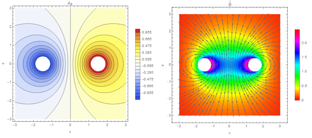
    H = {-D[Us[x, y], y], D[Us[x, y], x] + Us[x, y]/x}; {ContourPlot[Us[x, y], {x, y} \[Element] \[ScriptCapitalR]p, 
         Contours -> 20, FrameLabel -> {"x", "z"}, PlotRange -> All, 
         PlotLabel -> "\!\(\*SubscriptBox[\(A\), \(\[Theta]\)]\)", 
         PlotLegends -> Automatic, ColorFunction -> "TemperatureMap", 
         PlotPoints -> 50],StreamDensityPlot[H, {x, y} \[Element] \[ScriptCapitalR]p, 
          PlotRange -> All, 
          PlotLabel -> "\!\(\*OverscriptBox[\(B\), \(\[Rule]\)]\)", 
          FrameLabel -> {"x", "z"}, AspectRatio -> Automatic, 
          StreamPoints -> Automatic, StreamScale -> Automatic, 
          ColorFunction -> Hue, PlotLegends -> Automatic]}

Because I want to represent de potential vector and the magnetic field of a toroid, please if you know the answer, it would very usefull for me.

Yes! But it has circular section

Toroidal inductor?

YOu will need to apply the Coordinate Transformations . This is because the plot only works in Cartesian and Polar coordinates.

We have considered the case of a permanent magnet. In the case when there is an electric current in the loop, the vector potential should be used, then the equation will be different.

Thas exactly what I was trying thank you very much