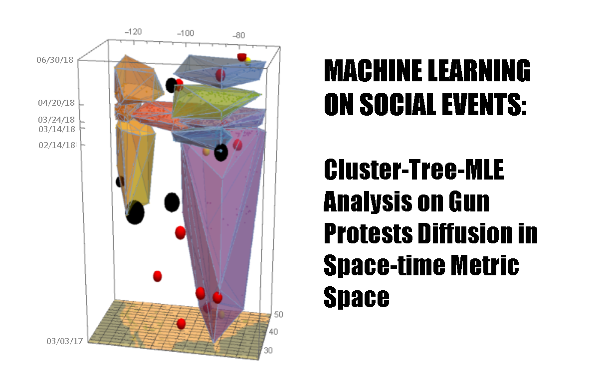
Project Title: Machine Learning on Social Events: Cluster-Tree-MLE Analysis on Gun Protests Diffusion in Space-time Metric Space
Also on: WordPress
Source Code and Data: GitHub repository
Executive Summary
This project studies the diffusion pattern of gun-control protests, using the method of space-time metric space which combines temporal and spatial information. The study finds that there is a significant relationship between the boundary of protest clusters and mass shooting cases. Inside each cluster, the jump pattern can be fitted by an exponential distribution. There are two main drivers in the diffusion of protest: geographical diffusion and burst, acting in the long and short timeframe respectively. It is expected that the cluster-tree-maximum likelihood estimation (MLE) approach for diffusion can be applied to the other areas of diffusion studies, including social practices or fields such as contagious diseases.
Introduction
Protests for stricter gun control have gained momentum since Donald Trump took office in 2017. The shooting in February 2018 at Marjory Stoneman Douglas High School and the national walk-out protests set off another wave of gun control protests that take place in various high schools and colleges across the country. Diffusion refers to the spread of something within a social system, previous research has established that different practices would spread in a region inside the society (Strang and Soule, 1998). Specifically for protest events, previous ones would have enlightenment and encouragement effect to subsequent events, and that geographical factor plays a key role in the spread of movements (Andrews and Biggs, 2006; Reising, 1999).
Image 0: Diffusion of gun protests in 2017 and 2018 in Western US.
Raw Data and Geographical Information Retrieving
Main folder: 1 - Data Retrieving
This project utilizes data from Count Love for protests and Mass Shooting Tracker (MST) for mass shootings. Count Love is a new database founded by researchers at Boston University and MIT, and MST is a database featured by CNN, MSNBC, The New York Times, The Washington Post, The Economist and more. They are both crowd-sourced database, which is a sensible choice of data for this project, especially when the Congress is not funding on gun-violence data and researches.
This project will focus on gun protests from March 2017 to the first half of 2018 in the Continental United States, thus Alaska, Hawaii, and other overseas territories would be excluded from this study. Based on the location information of the original data, geographical information (e.g. latitude/longitude/county etc.) would be retrieved by GeoPosition, GeoNearest, Interpreter?and other Entity-related-functions of Wolfram Language.
Points of Protest in the space-time metric space
Main notebook: 2 - analysis - Main.nb
We have the latitude, longitude and time of each data point. We put them together to form a space-time metric space. In mathematics, a metric space $(M, d)$ is a space with distance measure $d$, which can map each pair of points in $M$ into a real number, that is,
$$d: M \times M \rightarrow \mathbb{R}$$
where $d$ fulfills some requirements of having geometric meaning. Therefore we can use a unified distance function $d$ for both time and space. To visualize the space-time metric space, we can plot a 3D scatter plot by using Plot3D in Wolfram Language, together with a map of US which is imported by GeoGraphics at the respective coordinates range. We will then see a "vessel-shaped" U.S. with "clouds of dust" as her constituents, and the plot looks like a 3D nebula map in astrophysics.
Image 1: The "nebula" of gun protest in continental United States since March 2017 in the space-time crystal, which includes more than 2,600 protests.
There are more than 2,600 gun-related protests since March 2017. As we can see, the number of protests rockets since the notorious mass shooting in Parkland on February 14, 2018, and there are three large subsequent waves of protests up to April, namely the School Walkout (i.e. March 14), the March for Our Lives (i.e. March 24) and the 19th anniversary of the Columbine High School massacre happened in 1999 (i.e. April 20).
Cluster Analysis
As mentioned, by putting space and time in the metric space $(M, d)$, we are now able to define a united distance function [latex]d[/latex] to measure the protests occurrences in a time/space compounded sense.
One of the major considerations is the corresponding length of spatial distance compared to a specific period of time (namely $r$, i.e. $N$ degree of latitude v.s. one year). This would affect the scale between space and time in the distance function, as we will use Euclidean Distance in our subsequent study.
This ratio $r$ needs to make sense in the rate of diffusion. In the event history analysis of sociology, there is a sociological hypothesis that as a protest occurred in one locality, people there could inform and encourage their acquaintances elsewhere, who in turn could be inspired to initiate protest (Andrews and Biggs, 2006). We would, therefore, look at the normal practices of people's traveling inside the continent in their daily life for the space-time ratio $r$ justification.
It is normal for individual citizens to physically travel from county to the neighboring county within a single day, for meeting their acquaintances or transporting resources. It is, therefore, reasonable to use 33 miles (which is considered as the average distance between counties; justified in the file 0.2 - counties distance.nb) per day as our ratio $r$. In this study, we would use degree (i.e. latitude and longitude) instead of miles as the spatial measure, which would be much more efficient in converting between the geographical info in data and the distance for the subsequent quantitative analysis. And thus we would take $r$ to be 175 degrees per year (justified in 0.2 - counties distance.nb again).
In machine learning, cluster analysis is a technique to group a set of objects. We would then apply the clustering technique to the data, i.e. FindClusters. We would use Euclidean distance for the clustering analysis, as it is more sensible than other abstract mathematical metrics in real life. We would specify DistanceFunction -> EuclideanDistance as below, where {1,-2,-1} are the respective columns for the time-latitude-longitude triple:
cts = FindClusters[data[[All, {1, -2, -1}]] -> data[[All]], DistanceFunction -> EuclideanDistance]
This machine learning algorithm of FindClusters will find out the optimal number of clusters based on maximized likelihood. After doing the above, the protests are now separated into nine different clusters. We would further visualize it by using ConvexHullMesh in Wolfram Language as below, where colCts and n are the clusters and the number of clusters:
plot3 = Table[{HighlightMesh[ConvexHullMesh[ctsSel[[i]]], Style[2, colCts[[i]], Opacity[0.5]]]}, {i, n}];
Image 2: The "nebula" of gun protests are now separated into nine different clusters, which are first visualized in ellipsoids, and then in convex hulls
Mass Shooting Cases
We will look into each cluster to see the diffusion pattern of gun protests. Before doing so, we would study the relationship between protest and mass shooting in the sense of the cluster analysis. There are more than 500 mass shooting cases in the country since March 2017. There is a threshold model theory in statistical modeling, which states that some threshold value could be significant while the behavior of the model can vary in some important way before and after the threshold value.
Analytically speaking, it is reasonable to assume that the most severe cases would draw the attention of the public much more than the smaller one, and we would thus filter out the shooting bases by the number of people being killed/wounded for the subsequent study. We would use BubbleChart3Din Wolfram Language for the visulization.
Image 3: A 3D scatter-plot illustrating mass shooting cases. The size of spots reflects the number of people being killed in each case.
Relationship between protests and mass shooting in clustering sense
We then combine the plot of protests' clusters and the plot of the severe mass shooting cases to form the following 3D plot. We can see that there is a significant relationship between significant shooting events and the lower boundary of the clusters. The spots of mass shooting touch the bottom of the clusters, seemingly supporting the floating megaliths. Regarding the cluster of the waves in March 2018, we can see that the black spot (i.e. Parkland) and several red spots support the clusters from the ground up.
Image 4: Gun protest clusters and the mass shooting cases. The spots of mass shooting touch the bottom of the clusters, seemingly supporting the floating megaliths.
Tree of diffusion
In each cluster, we would apply techniques in graph theory to construct the network between the data points (i.e. the protests), and try to figure out how the practices of protest "jump" from one space-time duple (i.e. the latitude-longitude-time triple) to another duple (i.e. the spread inside the cluster). In graph theory, a spanning tree $T$ of an undirected graph $G$ is a subgraph that is a tree which includes all of the vertices of $G$, with the minimum possible number of edges. We would use the functions DelaunayMesh and FindSpanningTree as below, where ctsSelJ is the j-th cluster:
graph = IGMeshGraph@DelaunayMesh[ctsSelJ];
plot5 = FindSpanningTree[graph, VertexCoordinates -> GraphEmbedding@graph, EdgeShapeFunction -> "Line", EdgeStyle -> {Thick, Black}, VertexSize -> Tiny, VertexStyle -> Black, PlotTheme -> "Default"];
Thus the spanning tree would be a sensible candidate for network construction between protests if we are studying the geographical spread inside the cluster. Under the context of spanning trees, we would assume that the points of protests are "infected" by one of their nearest neighbors. The nine clusters would have their own spanning tree as below:
Image 5: Spanning tree of the nine clusters. The points of protests are "infected" by one of their nearest neighbors.
Jump Modeling by maximum likelihood estimation (MLE)
Each edge of the tree refers to a "jump" from one protest to another protest. Thus the jump would reflect the temporal and spatial distance differences between the previous and the next protest directly linked to the former. We would then try to model the temporal and spatial jumps by observing the statistics of jumps. We would like to focus on the spatial factor as a whole, and thus would combine latitude and longitude jump on Euclidean sense by $\Delta s = \sqrt{\Delta Lat^{2} + \Delta Long^{2}}$ for further processing. From the shape of the probability density function (PDF), we would assume that the spatial jumps of each cluster follow the Exponential Distribution $Exp(\lambda)$, whose PDF is given as below:-
$$f(x; \lambda)=\begin{cases}\lambda e^{-\lambda x}, \quad x\geq 0,\\ 0, \qquad \quad x<0. \end{cases}$$
Then we would obtain the $\lambda$ of each cluster by maximum likelihood estimation (i.e. MLE; EstimatedDistribution in Wolfram Language) as below, where ?1 and ?2 are the spatial and temporal parameters of the respective exponential distributions:-
distml = Table[EstimatedDistribution[edgeVectorsAllJ[[j, All, i]], ExponentialDistribution[?]], {i, 1, 2}];
{?1, ?2} = 1/Mean /@ distml;
Image 6: Probability comparison of "spatial jump" v.s. normal distribution and the respective PDF for the nine clusters. There is also the PDF curve of the fitted exponential distribution Exp(?) which is given by the maximum likelihood estimation.
Probability comparison of "spatial jump" v.s. normal distribution and the respective PDF for the nine clusters. There is also the PDF curve of the fitted exponential distribution Exp(?) which is given by MLE.
For the temporary factor, we would model it with a similar approach. We would assume the temporary and spatial factors are independent of each other.
Prediction of Gun Protests
Based on the occurred protest and the jump model obtained above, we can, therefore, make a prediction on the next protests based on the occurred events. At any specific time point $t_ 1$ (say, one day away from the latest data), we would have a "cross section" at $t_ 1$, which can be considered as a $t_ 1$-surface, namely $L_ {t_ 1}$. For every location $(lat_ i,long_ i,t_ 1)$ on $L_ {t_ 1}$, there will be temporal and spatial distances from it to the a respective nearest protest point. We would then subsequently obtain the PDF for the entire $L_ {t_ 1}$. Below is our protest prediction in the first few days in July 2018, based on the data up to June 30, 2018. We can see that Florida is most likely to have gun protests in early July 2018.
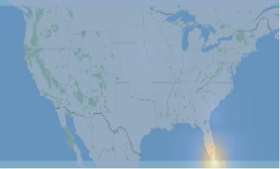
Image 7: Gun protests prediction in the first few days of July 2018, based on the data up to June 30, 2018. We can see that protests are most likely to happen in Florida in early July 2018.
To validate the model, protest data from July 1 to 5, 2018 from Count Love are used. There are two gun protests in the data, and below is the respective plot:-
Image 8: Validation of prediction model by using protest data from July 1 to 5, 2018. There are two gun protests in the data.
The protest on July 1 is exactly in Florida, and the next one is also located in the southern US.
Geographical Visualization
Main notebook: 3 - GeoListPlot.nb
To visualize the diffusion effect, we would look at each cluster to see how the protest spread inside the cluster at the county level. GeoListPlot would be applied to each of the nine clusters as below, which #[[1]] , #[[-4]], #[[-3]] are the columns of time, county and states respectively, while ctsI is the i-th cluster, and gr is the maximum graphical range to be fixed:
listTimeCountyI = {#[[1]], Entity["AdministrativeDivision", {#[[-4]], #[[-3]], "UnitedStates"}]} & /@ ctsI
GeoListPlot[Select[listTimeCountyI, #[[1]] <= date &][[All, 2]], GeoRange -> gr, GeoProjection -> "CylindricalEqualArea"]
Below is a cluster spanning October 2017 to March 2, 2018 in the US West coast:-
Image 9a: Spread of gun protests at the county level of a cluster. A pattern of geographical diffusion is observed.
We can see that it is very likely for the neighboring county to be "infected" and have follow-suit in protests. The geographical pattern within the region can be observed. The above GeoListPlot is only up to March 2, 2018, which is before the three big waves (the first is the school walk out on March 14, 2018) of gun protests in Spring 2018. The observation on geographical diffusion reflects the hypothesis of the proximity of social network (Andrews and Biggs, 2006) mentioned in the introduction. It is worth to point out that the timeframe of this process is relatively longer than the process mentioned below.
Below is another cluster which is located at the "time of waves" from March 3 to March 31, 2018, in the western US. We can see that when the waves (i.e. March 14 and 24, 2018) arrived, there are bursts of protests.
Image 9b: Bursts are observed in another cluster.
The geographical factor is much less significant than in the first geographical plot at the time of those bursts. Besides, the burst is referring to a shorter time frame. We would expect that the spread in this manner is due to a much faster flow of information, i.e. the internet.
We now look at another cluster locating at the Eastern US, which spans across both the "pre-waves period" and the "waves-period". Again, we can see some geographical diffusion before the waves, while there is no geographical significant observation during the burst.
Image 9c: A cluster which spans across both the "pre-waves period" and the "waves-period"
We can conclude that there are two main drivers of the protest: geographical diffusion and the burst, acting on two different timescales. To explain the pattern of protest spread, both the geographical diffusion and burst factor should be considered and be modeled to provide a coherent view of the whole picture.
Prediction for mass shooting
This project applies cluster-tree-MLE machine learning technique to the study of gun-control protests. In fact, with this cluster-tree-MLE technique, we can study the mechanism of any contagious process. The same technique can also be applicable to mass shooting cases with the MST's data.
Below is a prediction on the mass shooting cases in and after July 2018 based on the above cluster-tree approach with MST's data up to June 2018. Due to the statistical result, diffusion of mass shooting cases would act on an even longer timeframe, and thus validation of mass shooting would not be validated as of the writing on July 8, 2018.
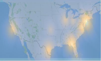
Image 10: Prediction on the mass shooting cases in and after July 2018 based on cluster-tree approach with MST's data up to June 2018.
Future work
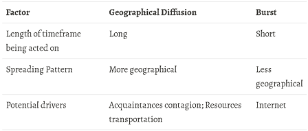
As mentioned above, there are two drivers on diffusion within the cluster, namely geographical diffusion and burst, each operating on long and short timeframe respectively. To explain the pattern of protest spread, both geographical diffusion and burst factors should be considered and modeled to provide a coherent view of the whole picture. In the future, we would try to figure out how to separate the two factors from the data. It is expected that the former can be processed by the similar tree-MLE approach, while the latter can be processed further by time series.
It is expected that the cluster-tree-MLE approach for diffusion can be applicable to the other areas regarding contagion, including social practices or fields such as contagious diseases. More future studies to apply the technique to those areas can be done.
Conclusion
To conclude, we have used cluster analysis with Euclidean distance on the time-space metric space of the gun protests events. There are nine clusters in the continental United States from March 2017 to June 2018. There is a significant relationship between the bottom boundary of the clusters and the severe mass shooting cases.
Inside each cluster, we have used spanning tree to construct the network between protest. After reviewing the statistics of the tree's edge, we would conclude that the jump can be basically fitted by an exponential distribution. A prediction model can be constructed based on the exponential distributions of the clusters.
The factors of protest diffusion can be separated into two types of main drivers: geographical diffusion and burst, respectively acting in the long and short timeframe. Their difference can be summed up in the below table:
References and Source Code
Source Code and Data: GitHub repository
Andrews, K. and Biggs, M. (2006). The Dynamics of Protest Diffusion: Movement Organizations, Social Networks, and News Media in the 1960 Sit-Ins. American Sociological Review, 71(5), pp.752-777.
Cohen, J. and Tita, G. (1999). Diffusion in Homicide: Exploring a General Method for Detecting Spatial Diffusion Processes. Journal of Quantitative Criminology, 15(4), pp.451-493.
Lohmann, S. (1994). The Dynamics of Informational Cascades: The Monday Demonstrations in Leipzig, East Germany, 198991. World Politics, 47(01), pp.42-101.
Reising, U. (1999). United in Opposition A Cross-National Time-Series Analysis of European Protest in Three Selected Countries. Journal of Conflict Resolution, 43(3), pp.317-342.
Strang, D. and Soule, S. (1998). Diffusion in Organizations and Social Movements: From Hybrid Corn to Poison Pills. Annual Review of Sociology, 24(1), pp.265-290.
Other Information
 Attachments:


