Generally it is always a good idea to provide working code so that others have a starting point.
All this is very easy to do in Mathematica. No need to use Excel either, because I see that you build analytic surfaces that can be sampled in Mathematica too.

First I recommend reading
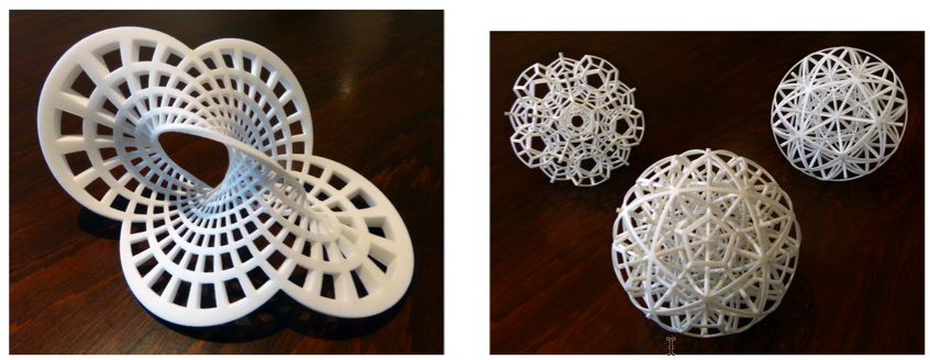
Notes on 3D printing by
Henry Segerman who did a lot of work on the subject and
published a paper.
A rather quick summary for you about specifically your problem. Here is the code:
f[u_, v_] := {u, v, u^2 - v^2};
scale = 40;
radius = 0.75;
gridSteps = 10;
curvesU = Table[scale*f[u, i], {i, -1, 1, 2/gridSteps}];
curvesV = Table[scale*f[j, v], {j, -1, 1, 2/gridSteps}];
tubesU = ParametricPlot3D[curvesU, {u, -1, 1},
PlotStyle -> Tube[radius], PlotRange -> All];
tubesV = ParametricPlot3D[curvesV, {v, -1, 1},
PlotStyle -> Tube[radius], PlotRange -> All];
corners =
Graphics3D[
Table[Sphere[scale f[i, j], radius], {i, -1, 1, 2}, {j, -1, 1, 2}]];
output = Show[tubesU, tubesV, corners]
Export["MathematicaParametricSurface.stl", output]
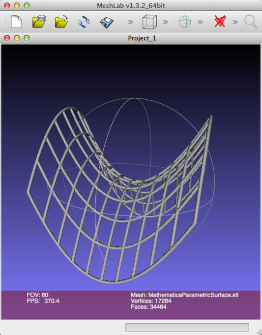
Here is how the resulting STL file is viewed in an independent STL viewing program - for example
MeshLab which is free:

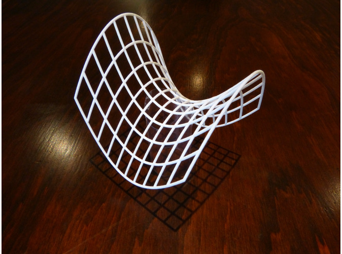
And here is final 3D printed
result you can find in Shapeways store:

Now sometimes you will wish to plot surfaces as they are, not as meshes. Here is a simple example.
model = RevolutionPlot3D[{Sin[t] + Sin[5 t]/10,
Cos[t] + Cos[5 t]/10}, {t, 0, Pi},
RegionFunction -> (Sin[5 (#4 + #5)] > 0 &), Mesh -> None,
BoundaryStyle -> Black, PlotStyle -> Thickness[.1]]
Export["model.stl", model];
Import[%]

Now further very useful links: