Message Boards Message Boards

0
|
7219 Views
|
9 Replies
|
7 Total Likes
View groups...
Share
Share this post:

Find second derivative using D?

Posted 6 years ago

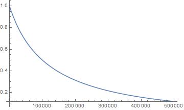
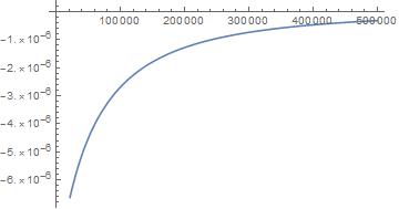
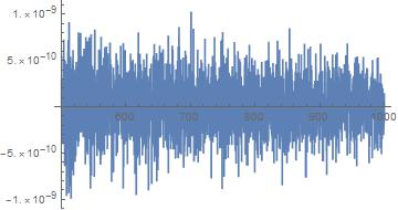
The code below gives incorrect 2nd derivative. figure 1 shows the original function xxSumS1[s, r] = funDervtveLAB[s, r, 0] when r=200, while second figure shows the 1st derivative of the original function "Exp[-noisepows]laplaceLABs[s, r]" when r=200. The 1st derivative is correct as the 1st derivative of a decreasing function is negative (figure 2). However, the 2nd derivative "xxSumS3[s, r] = funDervtveLAB[s, r, 2] when r=200" seems to be incorrect. This is because I expect it to be positive for all values of s as it is the derivative of the 1st derivative and the 1st derivative is an increasing function in s. Figure 3 shows the 2nd derivative of the original function

figure 1 figure 2 figure 3

    Clear["Global`*"]
    a = 4.88; b = 0.43; etaLAB = 10.^(-0.1/10); etaNAB = 10.^(-21/10); etaTB = etaNAB;
    PtABdB = 32; PtAB = 10^(PtABdB/10)*1*^-3; PtTBdB = 40; PtTB = 10^(PtTBdB/10)*1*^-3;
    NF = 8; BW = 1*^7; noisepowdBm = -147 - 30 + 10*Log[10, BW] + NF;
    noisepow = 0; RmaxLAB = 20000;

    TBdensity = 1*^-6; ABdensity = 1*^-6;
    alfaLAB = 2.09; alfaNAB = 2.09; alfaTB = 2.09;

    mparameter = 3;

    zetaLAB = PtAB*etaLAB; zetaNAB = PtAB*etaNAB; zetaTB = PtTB*etaTB;

    height = 100; sinrdBrange = -10; sinr = 10.^(sinrdBrange/10);

    probLoSz[z_] := 1/(1 + a*Exp[-b*(180/Pi*N[ArcTan[height/z]] - a)]);
       probLoSr[r_] := 1/(1 + a*Exp[-b*(180/Pi*N[ArcTan[height/Sqrt[r^2 - height^2]]] - 
              a)]);
      funLoS[z_] := z*probLoSz[z];
      funNLoS[z_] := z*(1 - probLoSz[z]);

    funLABNABs[z_, s_] := (1 - 1/(1 + s*zetaNAB*(z^2 + height^2)^(-alfaNAB/2)))*funNLoS[z];
    funLABLABs[z_, 
       s_] := (1 - (mparameter/(mparameter + s*zetaLAB*(z^2 + height^2)^(-alfaLAB/2)))^mparameter)*funLoS[z];
    funLABTBs[z_, s_] := z*(1 - 1/(1 + s*zetaTB*z^(-alfaTB)));

    distnceLABNABs = (zetaLAB/zetaNAB)^(1/alfaLAB)*height^(alfaNAB/alfaLAB);

    NearstInterfcLABNABs[r_] :=  Piecewise[{{height,  r <= distnceLABNABs}, {(zetaNAB/zetaLAB)^(1/alfaNAB)* r^(alfaLAB/alfaNAB), r > distnceLABNABs}}];
    NearstInterfcLABTBs[r_] := (zetaTB/zetaLAB)^(1/alfaTB)*r^(alfaLAB/alfaTB);
    NearstInterfcLABLABs[r_] := r;

    lowerlimitLABNABs[r_] := Sqrt[NearstInterfcLABNABs[r]^2 - height^2];
    lowerlimitLABLABs[r_] := Sqrt[NearstInterfcLABLABs[r]^2 - height^2];
    lowerlimitLABTBs[r_] := NearstInterfcLABTBs[r];

    InteglaplaceLABNABs[s_?NumericQ, r_?NumericQ] := NIntegrate[funLABNABs[z, s], {z, lowerlimitLABNABs[r], RmaxLAB}];
    InteglaplaceLABLABs[s_?NumericQ, r_?NumericQ] := NIntegrate[funLABLABs[z, s], {z, lowerlimitLABLABs[r], RmaxLAB}];
    InteglaplaceLABTBs[s_?NumericQ, r_?NumericQ] :=  NIntegrate[funLABTBs[z, s], {z, lowerlimitLABTBs[r], RmaxLAB}];


    laplaceLABNABs[s_, r_] :=  Exp[-2*Pi*ABdensity*InteglaplaceLABNABs[s, r]];
    laplaceLABLABs[s_, r_] := Exp[-2*Pi*ABdensity*InteglaplaceLABLABs[s, r]];
    laplaceLABTBs[s_, r_] := Exp[-2*Pi*TBdensity*InteglaplaceLABTBs[s, r]];
    laplaceLABs[s_, r_] := 
      laplaceLABNABs[s, r]*laplaceLABLABs[s, r]*laplaceLABTBs[s, r];

    funDervtveLAB[s_, r_, kk_] :=  D[Exp[-noisepow*s]*laplaceLABs[s, r], {s, kk}];

    xxSumS1[s_, r_] = funDervtveLAB[s, r, 0]; (*original function*)
    xxSumS2[s_, r_] = funDervtveLAB[s, r, 1];  (* 1st derivative*)
    xxSumS3[s_, r_] = funDervtveLAB[s, r, 2];  (*2nd derivative*)

    xxSumR1[r_] := xxSumS1[s, r] /. s -> (mparameter*sinr/zetaLAB*r^alfaLAB);
    xxSumR2[r_] := xxSumS2[s, r] /. s -> (mparameter*sinr/zetaLAB*r^alfaLAB);
    xxSumR3[r_] := xxSumS3[s, r] /. s -> (mparameter*sinr/zetaLAB*r^alfaLAB);
POSTED BY: mohamed alzenad
9 Replies

Mohamed,

The problem you are having is that you are doing a numerical calculation and running out of precision. Numerical derivatives are noisy operations -- you must maintain extreme precision to take multiple derivatives. Your calculation involves a Numerical integrate and then you take the derivative of it. I recommend taking the derivative analytically -- it will also speed things up. Another way to do this is to keep precision with Interpolation functions:

fun = Table[{x, xxSumS1[x, 200]}, {x, 0, 500000, 1000}];

(This is a bit slow but you can lower the resolution. Also, You will get warnings which you can fix by specifying AccuracyGoal in the NIntegrate)

ifun = Interpolation[fun]
Plot[ifun[x], {x, 0, 500000}]
Plot[ifun'[x], {x, 0, 500000}]
Plot[ifun''[x], {x, 0, 500000}]

To get

enter image description here

POSTED BY: Neil Singer

Your calculations use NIntegrate, a numerical method. Symbolic differentiation cannot handle a numerical function.

POSTED BY: John Doty

Mohamed,

to do the 2D interpolation I recommend the following:

  1. Use fewer points in x because the function is fairly flat in that direction (see the 3D Plot below) to save time
  2. Chop off small imaginary parts (some solutions with x or y 0 have infinitesimal imaginary parts)
  3. Reformat the data into the correct format for interpolation and plotting by Flattening the table.

    funTable2D = Table[{x, y, xxSumS1[x, y]}, {x, 0, 500000, 10000}, {y, 0, 500000, 1000}];
    funTable2Dc = Flatten[Chop[funTable2D], 1];
    

View the result:

ListPlot3D[funTable2Dc]

enter image description here

Now you can do the interpolation:

ifun2D = Interpolation[funTable2Dc]

To Plot

Plot[ifun2D[x, 200], {x, 0, 500000}]

Derivatives

fun2 = D[ifun2D[x, y], x]
fun3 = D[ifun2D[x, y], {x, 2}]

To Plot:

Plot[fun2 /. y -> 200, {x, 0, 500000}]
Plot[fun3 /. y -> 200, {x, 0, 500000}]

I hope this help.

Regards,

Neil

POSTED BY: Neil Singer

Mohamed,

I am guessing that your issue is related to numerical precision and your use of spline interpolation. If you want to take multiple derivatives (which is a highly noisy process) you will need to set your interpolation order high enough to be able to take derivatives (which successively get worse.) Spline interpolation makes for a smooth function that is forced to go through all of the data points. Numerically the splining process can result in strange artifacts (like the function looping around to go through a point). Therefore, the spline interpolation is unlikely to give good derivatives. Try using a higher order (but not spline) interpolation. But understand your function and what you are doing is running into numerical precision/instability issues.

Let me know if the interpolation change helps.

Regards,

Neil

POSTED BY: Neil Singer

Thank you John for your reply. The numerical integration is with respect to the variable z and it gives a function in s and r, for example; InteglaplaceLABNABs[s,r] is a function in s and r.

InteglaplaceLABNABs[s_?NumericQ, r_?NumericQ] := NIntegrate[funLABNABs[z, s], {z, lowerlimitLABNABs[r], RmaxLAB}];

I used D on NIntegrate for the 1st derivative and it worked well and gave good result.

POSTED BY: mohamed alzenad

Thank you Dr Neil Singer for the reply. As suggested by Dr Neil Singer , for a given r=200, the following code works well

 funTable = Table[{x, xxSumS1[x, 200]}, {x, 0, 500000, 1000}];
    ifun = Interpolation[funTable]
    Plot[ifun[x], {x, 0, 500000}]
    Plot[ifun'[x], {x, 0, 500000}]
    Plot[ifun''[x], {x, 0, 500000}] 

Now, I want to generalize it for any value for r. So, I did interpolation in 2-D. The above code becomes

funTable2D = Table[{x, y, xxSumS1[x, y]}, {x, 0, 500000, 1000}, {y, 0, 500000, 1000}];
ifun2D = Interpolation[funTable2D]
Plot[ifun2D[x, 200], {x, 0, 500000}]
Plot[ifun2D'[x, 200], {x, 0, 500000}]
Plot[ifun2D''[x, 200], {x, 0, 500000}]   

The above code takes a long time to do the interpolation. Any suggestion that may help is really appreciated.

POSTED BY: mohamed alzenad

Any help in solving this is really appreciated

POSTED BY: mohamed alzenad

Thank you Neil, I tried your suggestions above and worked well for up to the 3rd derivative. For the 4th derivative, the value of "ExactCondCovegeProbLAB22" is a negative large number which is not correct because it is a probability (it should be between 0 and 1). I plotted "funTable2D" and "ifun2D" to see how good the interpolation function "ifun2D" is as follows

ListPlot3D[funTable2Dc]

enter image description here

Plot3D[ifun2D[s, r], {s, LlimitxS, UlimitxS}, {r, LlimitxR, UlimitxR}]

enter image description here

As we can see, the two functions does not look similar

LlimitxR = height; UlimitxR = Sqrt[RmaxAB^2 + height^2];
LlimitxS = parmtrLAB[LlimitxR]; UlimitxS = parmtrLAB[UlimitxR];

Print[111];
funTable2D = 
  Table[{s, r, Exp[-noisepow*s]*laplaceLAB[s, r]}, {s, LlimitxS, 
    UlimitxS, 10000}, {r, LlimitxR, UlimitxR, 500}];
Print[222];
funTable2Dc = Flatten[Chop[funTable2D], 1];
Print[333];
ifun2D = Interpolation[funTable2Dc, Method -> "Spline"];
Print[444];
funDervtveLAB22[s_, r_, kk_] := (-s)^kk/kk!*D[ifun2D[s, r], {s, kk}];
xxSumS22[s_, r_] := 
  Sum[funDervtveLAB22[s, r, kk], {kk, 0, mLParm - 1}];
xxSumR22[r_] := xxSumS22[s, r] /. s -> (mLParm*sinr/zetaLAB*r^alfaLAB);
xxPdF22[r_] := xxSumR22[r]*CondPdfLAB[r];
ExactCondCovegeProbLAB22[[hIdx, mIdx]] = 
  NIntegrate[xxPdF22[r], {r, height, Sqrt[RmaxAB^2 + height^2]}];
POSTED BY: mohamed alzenad
Anonymous User
Anonymous User
Posted 5 years ago

Thanks to all of you for giving a lot of knowledge and clear the confusion

POSTED BY: Anonymous User
Reply to this discussion
Community posts can be styled and formatted using the Markdown syntax.
Reply Preview
Attachments
Remove
or Discard

Group Abstract Group Abstract