This thread is inspired by
the question about solving a wave function on the Wolfram Community. In Mathematica one uses
NDSolve plus some known boundary conditions and initial conditions to tackle this type of problem, just as Nasser's response in that thread.
In Wolfram System Modeler (WSM), two approaches are available: one mainly uses equation and the other is about building proper components. I will only talk about the first one because it is fairly very basic and a quick approach for simple systems.
The general 1-D wave equation is a fourth order PDE. I choose finite difference method to partition the spacial domain (along x-axis usually) and solve the
2nd order ODE on each section. In this example, I need array functionalities and the time derivative function (der) in the model.
The original problem is about numerically solving
the following equation with given boundary conditions (bc) and initical conditions (ic)
Suprisingly, the implementation of my scheme is fairly concise in the WSM (this is the ACTUAL* code, not pseudo code):
model waveFunctionModel
parameter Real ll=6.28319 "Length of the domain";
parameter Integer n=50 "number of partitions ";
parameter Real initdisp[n]={0.0,0.127877,0.253655,0.375267,...} "initial condition";
parameter Real initddisp[n]=zeros(n) "initial speed of each node";
parameter Real dx=ll/(n - 1) "length of segments";
Real ndisp[n](start=initdisp) "node displacement";
Real dndisp[n](start=initddisp) "node speed";
equation
der(ndisp[1:n])=dndisp[1:n];
for i in 2:n - 1 loop
der(dndisp[i])=(ndisp[i + 1] - 2*ndisp[i] + ndisp[i - 1])/dx^2;
end for;
ndisp[1]=time*sin(time);
ndisp[n]=0;
end waveFunctionModel;
Let's take a look at the details: The declarations and defintions of some parameters sit at the beginning of the code. I defined the parameters for the length of the space domain, number of nodes (n=50, results 49 segments).
parameter ll, n, dx ...
Also I have defined the initial profile of the object through initdisp, which is an array of 50 elements and gives the starting points of the nodes. The "Real ndisp" declares a list of variables (again 50 elements) that record the displacement of the each node. "dndisp", similarly, stand for the derivative of "ndisp" wrt time.
WSM is about interpretive programming language. In equations I just need to tell the relationship between variables instead of assignment. The line below generates a state vector,
der(ndisp[1:n])=dndisp[1:n];
which is equivalent to

The for-loop, from the next line, uses
a second order difference to represent the 2nd order partial derivative about x for all interior points across the domain. The last two lines here define the two boundary conditions at each end:
for i in 2:n - 1 loop
der(dndisp[i])=(ndisp[i + 1] - 2*ndisp[i] + ndisp[i - 1])/dx^2;
end for;
ndisp[1]=time*sin(time) " boundary condition at x = 0";
ndisp[n]=0 "boundary condition at x = 2 * Pi";
Besides, I want to test whether the code above generates correct result at the end of the simulation, I would like tocompare its output with that from NDSolve.
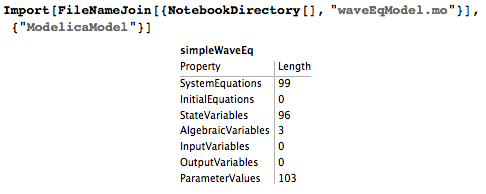
WSMLink package offers a collection of very handy functions so I can do it just inside Mathematica. I put the working notebook and the model in the same directory and I import it directly after I have loaded WSMLink package in Mathematica 8+
<<WSMLink`
Import[FileNameJoin[{NotebookDirectory[],"waveEqModel.mo"}],{"ModelicaModel"}]

WSMSimulate generates a compiled file, which would be runtime later. The "StateVariables" option can be set in
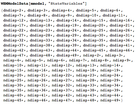
WSMModelData function to pick up a state variable or a node as output.Again, each ndisp means the nodal displacement of a given index and dndnisp means the speed of the node
mmodel = "simpleWaveEq";
\[ScriptCapitalM] = WSMSimulate[mmodel, {0, 10}]
WSMModelData[mmodel, "StateVariables"]

Based on the form of the output, I write the following subrouting to extract the proper state variables:
var[i_Integer] := ToExpression["ndisp\[LeftPointer]" <> ToString[i] <> "\[RightPointer]"];
Say I am interested in the displacement of node 10 over 10 seconds (or the default value of the entire simulation duration), which corresponds to x = "position" for y[x,t]
n = 10;
plt1 = WSMPlot[\[ScriptCapitalM], {Evaluate[var[10]]}, PlotStyle -> {Green, Thickness[0.012]}, PlotLegends -> Automatic];
position = (n - 1)*(6.28319)/49;
plt2=Plot[Evaluate[y[position,t]/.sol],{t,0,10},PlotStyle-> {Red},PlotLegends->Automatic];
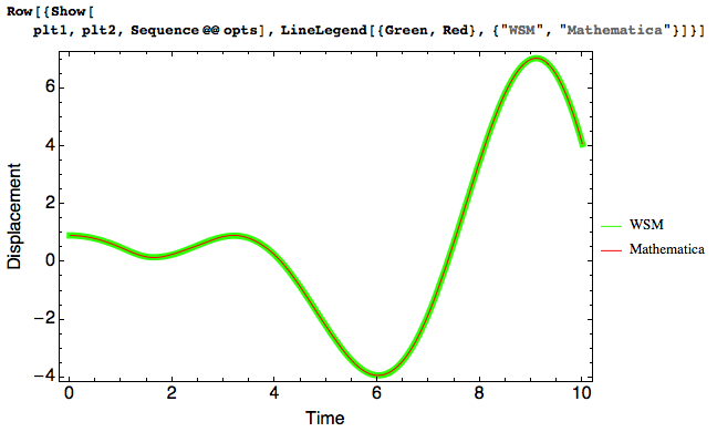
I put the two plots in the Show function wrapper plus some options** to beautify the results:The thin red line is the result from Mathematica NDSolve equation and the thick green line represents the simulation from WSM. They match perfectly as I have expected.
Row[{Show[plt1,plt2,Sequence@@opts],LineLegend[{Green,Red},{"WSM","Mathematica"}]}]

This is all I have done for this problem. Hopfully it is helpful for those interested in Wolfram System Modeler and in how it interacts with Mathematica.
Things you can try by yourself:
1) Change the initial value/ic of the model and input function/bc (hint: use "ParameterValues" in WSMModelData)
2) Use the model above and check the profiles of other nodes. Then compare them with the solution from Mathematica. (hint: change n from 1 to 50)
Notes:
*: initdisp has "..." in the list for the sake of line space. You can generate the piece of code for this particular initial condition:
N[Sin[Range[0, 2.*\[Pi], 2 \[Pi]/49]]]
**: the option varaible-opts-applied in the last show function is defined as:
opts={Frame->True,FrameLabel->{{"Displacement",None},{"Time",None}},LabelStyle-> Directive[16,FontFamily-> "Helvetica"],PlotRange->All,Axes->False};
***:
These steps (by Nasser) solve y[x,t] :
