In this post I'll share a Neural Network (NN) arquiteture capable of classifying a input image of a Cellular Automaton (CA). This input image can be of any dimension (width and height).
First we'll create a function called RandomRule capable of generating a random CA.
RandomRule[n_Integer, W_Integer, H_Integer] := Image[
    1 - CellularAutomaton[n, RandomInteger[1, W], H-1],
    ImageSize -> {UpTo@256, UpTo@256}
]
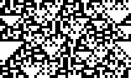
For example, RandomRule[90, 50, 30] gives:
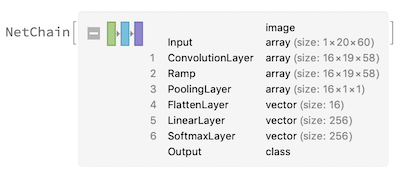
The NN arquiteture will consiste of 16 Convolutional Layers of with a kernel of 2x3 (height 2 and width 3). This kernel size is choosen because it fits the CA rules, where the three neighboors of a line determine the center cell of the line bellow. A Pooling Layer will colapse all spatial dimension of the result into a single tensor of length 16x1x1, which is a requirment to make the NN size-independendant, which will then be Flatten out and 256 Linear Layers will be used for classification using SoftMax.
net[W_Integer, H_Integer] := NetInitialize@NetChain[{
    ConvolutionLayer[16, {2,3}],
    Ramp,
    PoolingLayer[{H,W} - {1,2}],
    FlattenLayer[],
    LinearLayer[256],
    SoftmaxLayer[]
},
    "Input" -> NetEncoder[{"Image", {W, H}, "ColorSpace" -> "Grayscale"}],
    "Output" -> NetDecoder[{"Class", Range[0, 255]}]
]
The data to train the NN will be random CA image that map the rule it generate.
data[W_Integer, H_Integer, n_Integer] := Table[
    RandomRule[i, W, H] -> i
, {i, RandomChoice[Range[0,255], n]}]
Let's initialize a trained model 60x20, which is big enough but still fast:
trained = net[60, 20];
We will train the net:
trained = NetTrain[trained,
    data[60, 20, 256*128],
    MaxTrainingRounds -> 1000,
    BatchSize -> 256*4,
    TargetDevice -> "GPU"
]
After the error drops less than 0.5% we can stop the training and it will be saved automatically. You can re-train the model with new input by simply re-evaluating the cell above. In my machine (GTX 1050) it takes about 5min to train.
Let's classify how well does this NN does on new data (remember that the function data creates new data each time it is run).
cm = ClassifierMeasurements[trained, data[60, 20, 256*128]];
Quantity[100*cm["Accuracy"], "Percent"]
Output: 99.7498%
Which gives a very good mark for such a simple NN. I wont plot the ConfustionMatrix because it is very confusion, as a 256x256 matrix...
Now for the fun part. How can we use this NN to classify any input image of any size? We will recreate a NN as the previous one, but add the weigths and biases from the trained net (I tried NetReplacePart with no succes...).
netTrained[W_, H_] := NetChain[{
    ConvolutionLayer[16, {2, 3},
       "Weights" -> NetExtract[trained, {1, "Weights"}],
       "Biases" -> NetExtract[trained, {1, "Biases"}]
    ], Ramp,
    PoolingLayer[{H,W} - {1,2}],
    FlattenLayer[],
    NetExtract[trained, 5],
    SoftmaxLayer[]
},
    "Input" -> NetEncoder[{"Image", {W,H}, "ColorSpace" -> "Grayscale"}],
    "Output" -> NetDecoder[{"Class", Range[0, 255]}]
]
With the code bellow we can test different input sizes, where all the rules are evaluated for 50 random input images. The Union is used to avoid duplicated points.
Block[{W=70,H=20, netTemp, pts},
    netTemp = netTrained[W,H];
    pts = Flatten[Table[
       {i, netTemp[RandomRule[i, W,H]]}
    , {i,0,255}, {50}], 1] // Union;
    ListPlot[pts,
       FrameLabel -> {"Correct Rule", "Predicted Rule"},
       PlotLabel -> StringTemplate["`1` x `2`"][W,H]]
]
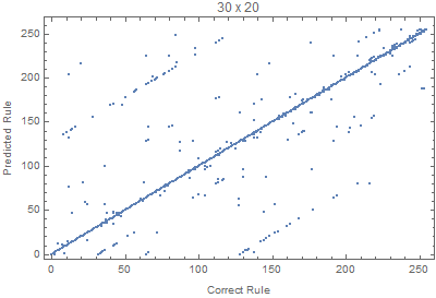
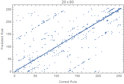

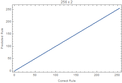
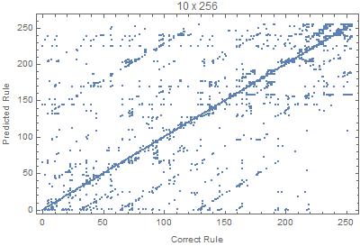
Where we can see that images with larger widths are more important, since it gives more variation, since lots of rules die down quickly with height.
The NN arquiteture could be easily scaled down for less convolutional layers and the output could be compressed from 256 one-hot, to 8-bits, to use less degrees of freedom (the current one uses 4464 elements).