Lets simulate some data distributed for example normally:
data = RandomVariate[NormalDistribution[3, 2.5], 10^4];
We can use so called SmoothKernelDistribution to build a general smooth distribution curve
SKD = SmoothKernelDistribution[data];
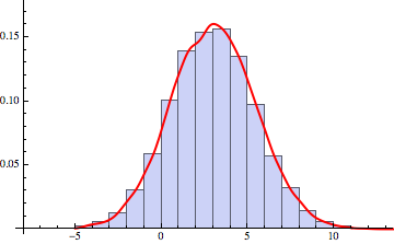
To show visually correspondence with data:
Show[Histogram[data, 20, "PDF"], Plot[PDF[SKD, x], {x, -5, 15}, PlotStyle -> Directive[Red, Thick]]]

But on other hand, if you would have a guess, what kind of known analytic distribution fits your case, you could try to find distribution parameters that fit your data best - and of course they are very close to the parameters we have chosen for original Gaussian to simulate your data:
params = FindDistributionParameters[data, NormalDistribution[a, b]]
Out[] = {a -> 3.00242, b -> 2.45767}
And you could check whether it is a good choice of distribution - in this case of course it is:
ND = NormalDistribution[a, b] /. params;
tstData = DistributionFitTest[data, ND, "HypothesisTestData"];
{tstData["AutomaticTest"], tstData["TestConclusion"]}

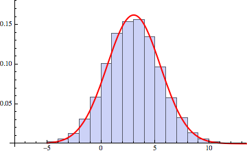
Plot:
Show[Histogram[data, 20, "PDF"], Plot[PDF[ND, x], {x, -5, 15}, PlotStyle -> Directive[Red, Thick]]]

Now you can easily find various probabilistic and statistical characteristics of this distributions:
Probability[5 < x < 10, x \[Distributed] SKD]
Out[] = 0.207631
Probability[5 < x < 10, x \[Distributed] ND]
Out[] = 0.205963
If you need a practical demonstration of this with real world data take a look at Vitaliys answer here:
Finding the actual wind power at a location for a given period?