It seems there's some problem when using
ColorFunction with a
StremDensityPlot and with its options on
StreamPoints:
I'm trying to create a demonstration (much more complex than the simple example posted here) in wich there are the field lines of an electric dipole and in the background there's a color representing the field intensity. But it seems that the StreamPoints settings affect the rendering of the background color (set through the option ColorFunction):
With this code
FieldPts =
Flatten[{Table[{{xq1 + d Cos[\[Alpha]], yq1 + d Sin[\[Alpha]]},
RGBColor[1, 1, 0]}, {\[Alpha], 0, 2 \[Pi] + 0.1, \[Pi]/(3 4)}],
Table[{{xq2 + d Cos[\[Alpha]], yq2 + d Sin[\[Alpha]]},
RGBColor[1, 1, 0]}, {\[Alpha], 0, 2 \[Pi] + 0.1, \[Pi]/(
3 4)}]}, 1] /. {xq1 -> -2, yq1 -> 0, xq2 -> 2, yq2 -> 0,
qq1 -> 2, qq2 -> -2, s -> 2, d -> 0.7};
mycolfunc[z_] :=
GrayLevel[
2/\[Pi] ArcTan[z]]; StreamDensityPlot[{-((
2 (-2 + x))/((-2 + x)^2 + y^2)^(3/2)) + (
2 (2 + x))/((2 + x)^2 + y^2)^(
3/2), -((2 y)/((-2 + x)^2 + y^2)^(3/2)) + (2 y)/((2 + x)^2 + y^2)^(
3/2)}, {x, -7, 7}, {y, -7, 7}, ColorFunction -> mycolfunc,
ColorFunctionScaling -> False, StreamPoints -> FieldPts]
I get this image:
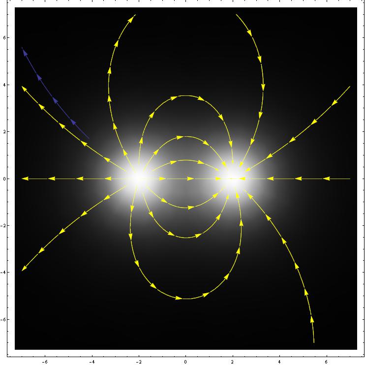
That's ok.
But if I add some other setting to the StreamPoint command (in the form of "
{spec,dspec,len}" to specify a minimum distance between streamlines and a maximum length for any streamline)...
FieldPts =
Flatten[{Table[{{xq1 + d Cos[\[Alpha]], yq1 + d Sin[\[Alpha]]},
RGBColor[1, 1, 0]}, {\[Alpha], 0, 2 \[Pi] + 0.1, \[Pi]/(3 2)}],
Table[{{xq2 + d Cos[\[Alpha]], yq2 + d Sin[\[Alpha]]},
RGBColor[1, 1, 0]}, {\[Alpha], 0, 2 \[Pi] + 0.1, \[Pi]/(
3 2)}]}, 1] /. {xq1 -> -2, yq1 -> 0, xq2 -> 2, yq2 -> 0,
qq1 -> 2, qq2 -> -2, s -> 2, d -> 0.7};
mycolfunc[z_] :=
GrayLevel[
2/\[Pi] ArcTan[z]]; StreamDensityPlot[{-((
2 (-2 + x))/((-2 + x)^2 + y^2)^(3/2)) + (
2 (2 + x))/((2 + x)^2 + y^2)^(
3/2), -((2 y)/((-2 + x)^2 + y^2)^(3/2)) + (2 y)/((2 + x)^2 + y^2)^(
3/2)}, {x, -7, 7}, {y, -7, 7}, ColorFunction -> mycolfunc,
ColorFunctionScaling -> False, StreamPoints -> {FieldPts, 1, 10}]
... then I get this
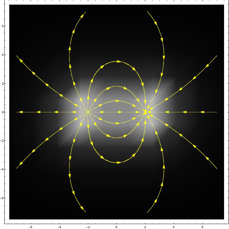
In this latter case the field intensity is clearly not as expected (it seems as there are cubes seen in perspectives... (?) )
Anyway I need the second kind of code to be able to set the number, length and density of the field lines.
I wonder why a simple change in this option can change the behaviour of the ColorFunction result.
The only working solution I could find was to overlap the StreamDensityPlot with a
blank DensityPlot with just the ColorFunction option in it. But I think that's not efficient and it can slow down my demonstration (in which there will be the possibility to move the source charges).
Any help, suggestion?
[
Edit - 11/11/2013: I can consider my question as [
Solved] with Shedelbower's hint about using the
MaxRecursion->2 (or more) option]


