Explore
Wolfram Demonstrations on the subject - a lot of free code to download and nice looking applications. For example:
Taylor Polynomials by Harry Calkins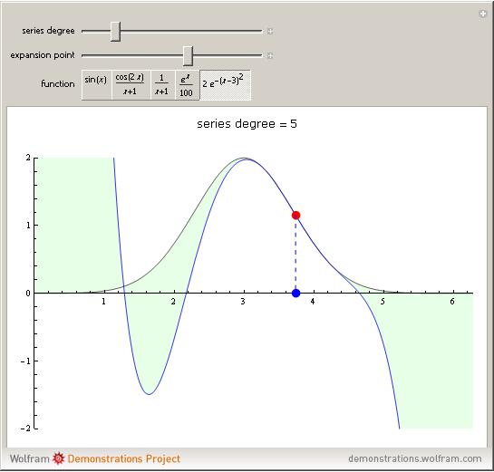
Manipulate[
Column[{Style[Row[{"series degree = ", deg}], "Label", 12],
Plot[Evaluate@{func /. x -> t,
MakeSeriesFunction[func, x, deg, pt]}, {t, 0, 2 Pi},
PlotRange -> {{0, 2 Pi}, {-2, 2}},
PlotStyle -> {{GrayLevel[.25, .85]}, {RGBColor[0, 0, .9, .8]}},
Filling -> {1 -> {{2}, Directive[{Opacity[.1], Green}]}},
Epilog -> {Red, PointSize[.02], Point[{pt, func /. x -> pt}],
Blue, Point[{pt, 0}], Dashing[{.01}],
Line[{{pt, func /. x -> pt}, {pt, 0}}]},
ImageSize -> {500, 350}]}, Center], {{deg, 10, "series degree"},
1, 24, 1}, {{pt, 0, "expansion point"}, 0,
2 Pi}, {{func, Sin[x],
"function"}, {Sin[x] -> TraditionalForm[Sin[x]],
Cos[x*2]/(x + 1) -> TraditionalForm[Cos[x*2]/(x + 1)],
1/(1 + x) -> TraditionalForm[1/(1 + x)],
E^x/100 -> TraditionalForm[E^x/100],
2 E^-(-3 + x)^2 -> TraditionalForm[2 E^-(-3 + x)^2]}},
SaveDefinitions -> True,
Initialization :> {MakeSeriesFunction[fn_, var_, deg_, pt_] :=
Module[{wrkfn},
wrkfn[tt_] =
If[Head[fn] === Symbol && fn =!= var, fn[tt], fn /. var :> tt];
Normal@Series[wrkfn[t], {t, pt, deg}]
]}]


