@Kampas created
a short thread about his work around in solving the following optimization problem
Minimize[{x^2 - y^2,
Reduce[{Cos[x - y] >= 1/2, -5 <= x <= 5, -5 <= y <= 5}, {x, y}]}, {x, y}]
Without using the Reduce function here, one would not have result. Short as it, Kampas's example in fact sheds light on the abstract words about the very advanced technology Mathematica:
symbolically enhanced numeric computing.
Let me quickly explain why Kampas's trick work : when you solve the optimization problem with the non-reduced version,
Minimize[{x^2 - y^2, Cos[x - y] >= 1/2, -5 <= x <= 5, -5 <= y <= 5}, {x, y}]
Mathematica will use the nonlinear constraints and try to look for the global minimum over a broken domain. This involves many tedious computation and jumpy steps, which are very bad for either symbolic or numeric steps. On the other hand, Reduce function breaks the domain into several linear pieces and join them thru Or[] operator. Then Mathematica automatically knows exactly what to do for these classic linear constrained quadratic programming problem. The smart mechanism for such numeric solving process is derived from its ultimate symbolic processing power.
To illustrate my point, I have inserted some dynamic and hacky code into Kampas's problem. You will see Mathematica can handle the same problem in two different way. I first just use simple graphics function to plot the target function across the valid domain
DensityPlot[x^2 - y^2, {x, -5, 5}, {y, -5, 5},
RegionFunction -> Function[{x, y, z}, Cos[x - y] >= (1/2)]
Then I use the NMinimize function along with StepMonitor option to extract the intermediate tracking points:
Reap[Minimize[{x^2 - y^2, Cos[x - y] >= 1/2, -5 <= x <= 5, -5 <= y <= 5}, {x, y},StepMonitor :> Sow[{x, y}]]]
where Reap and Sow help return the values. Finally, I use the Epilog option in the DensityPlot block to add a layer of tracking points over the density map of the target function. The actual Manipulate function looks lenthy because of the large option list. But the core is nothing more than the two pieces of code just mentioned.
Here comes the interesting thing. Even I force the solver to use exactly the same method, the graphics are always different depending on wheather Reduce function is added or not.
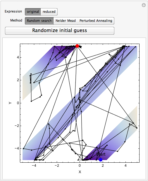
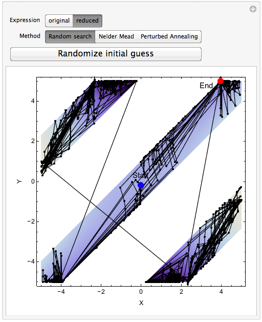
The blue dot and the red dot are the initial guess and the candidate minimum value, respectively. If we take a look at the two diagrams carefully, we notice several things:
1. The first diagram seems to have more points go across the gap than the second one
2 There are more points actually sits outside of the domain in the first diagram than those in the second one.
3. The points in the first diagram is random and does very few local check
4. The location for the minimum is different
These observation are quite similar even I switch methods:
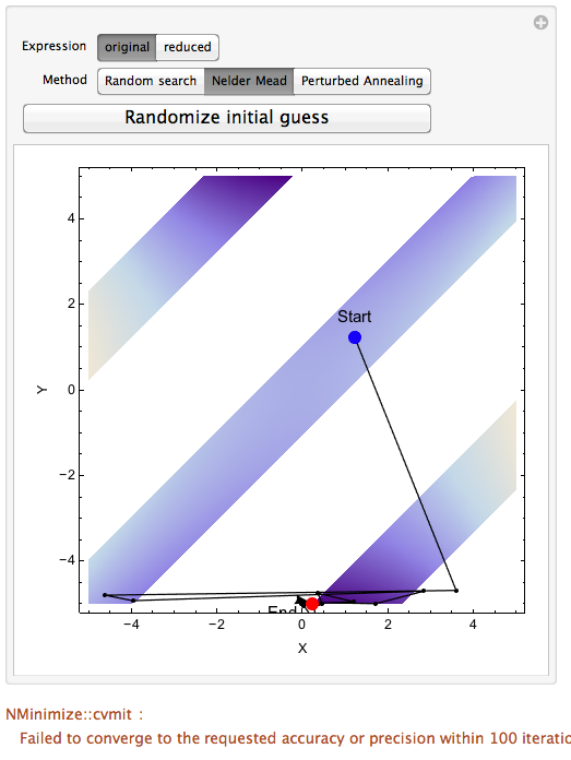
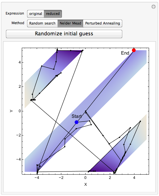
Just like I have briefly mentioned, the optimization solver indeed uses very different domains for the two cases. In the first situation where the trigonometric constraint is present, Mathematica's stochastic method does trial-and-error over the entire {-5,5}-by-{-5,5} plane. While in the second case, most computations are done within each band. Also if you play around with this Manipulate function by clicking the randomize button, you can see the "cvmit" convergence problem for non-reduced case. This means that this method is not stable for the non-reduced case.
Even though the reduced version might not always give the actual global minimum, we still prefer this way because the numeric stability for the expression itself.
Copyable code:
Manipulate[
res2 = Reap[
NMinimize[{x^2 - y^2,
expr /. {
"original" ->
Sequence[Cos[x - y] >= 1/2, -5 <= x <= 5, -5 <= y <= 5],
"reduced" ->
Reduce[{Cos[x - y] >= 1/2, -5 <= x <= 5, -5 <= y <= 5}, {x, y}]
}
}, {x, y},
Method -> (opts /. {
"Random search" ->
{"RandomSearch", "RandomSeed" -> k,
Method -> "InteriorPoint"},
"Nelder Mead" -> {"NelderMead", "ShrinkRatio" -> 0.95,
"ContractRatio" -> 0.95, "ReflectRatio" -> 2,
"RandomSeed" -> k},
"Perturbed Annealing" -> {"SimulatedAnnealing",
"PerturbationScale" -> 3, "RandomSeed" -> k }
}
), StepMonitor :> Sow[{x, y}]]
];
pts2 = res2[[2, 1]];
DensityPlot[x^2 - y^2, {x, -5, 5}, {y, -5, 5},
RegionFunction -> Function[{x, y, z}, Cos[x - y] >= (1/2)],
Epilog -> {
Arrow[pts2],
Join[{Point[pts2[[2 ;; -2]]]}, {{PointSize[0.03], Blue,
Point[pts2[[1]]]},
{PointSize[0.03], Red, Point[pts2[[-1]]]}
}],
Inset[Style["Start", 12], pts2[[1]] + {0, 0.5}],
Inset[Style["End", 12], pts2[[-1]] + {-0.7, -0.2}]
},
Mesh -> None,
FrameLabel -> {"X", "Y"}
],
{{expr, "original", "Expression"}, {"original", "reduced"}},
{
{opts, "Random search", "Method"},
{"Random search", "Nelder Mead", "Perturbed Annealing"}
},
Button["Randomize initial guess", k = RandomInteger[{1, 100}]]
]


