Hi Neil!
Ahh thanks for the infos with SysModeler, I'll most definitely have a look at it! and I signed up for the webinar ;) Look forward to seeing your presentation. Mathematica being able to program embedded processors will be a godsend. I'll wait to upgrade then :)
Ahh Since I couldn't figure out how to post the nonlinear state space model in the code, I'll post the entire thing up until the gains.
params = {m1 -> 0.2928, m2 -> 0.1102, l -> 0.087596, k -> 0.09,
   c1 -> 0.0089, c2 -> 0.00001,
   I1 -> (885.758 10^-6 + 0.087596^2*0.354),
   I2 -> (339.10 10^-6 + 130 10^-6 + 0.09^2 0.1102), \[Tau] ->
    33.5 10^-3, g -> 9.81 };
rparams = {\[Alpha] -> (I1 + I2 + l^2 m1 + k^2 m2), \[Beta] ->
    g (l m1 + k m2)} ;
Here are the system vectors to build the Lagrangian.
rx = l Sin[\[Theta][t]];
ry = -l Cos[\[Theta][t]];
sx = k Sin[\[Theta][t]];
sy = -k Cos[\[Theta][t]];
\[Tau]\[Theta] = I2 \[Omega]''[t];
\[Tau]\[Omega] = -\[Tau] u[t] + I2 \[Theta]''[t];
\[Eta]\[Omega] = c1 \[Omega]'[t];
\[Eta]\[Theta] = c2 \[Theta]'[t];
fx = -f[t] l Sin[\[Theta][t]];
fy = f[t] l Cos[\[Theta][t]];

T1 = 1/2 (m1 (D[rx, t]^2 + D[ry, t]^2) +
     I1 \[Theta]'[t]^2) (*pendulum body*);
T2 = 1/2 (m2 (D[sx, t]^2 + D[sy, t]^2) + I2 \[Theta]'[t]^2 +
     I2 \[Omega]'[t]^2)(*flywheel*);
V1 =  m1 g ry (*pendulum body*);
V2 =  m2 g sy (*fly wheel*);
Make the odes
eqn1 = FullSimplify[D[D[L, \[Theta]'[t]], t] - D[L, \[Theta][t]]]
eqn2 = FullSimplify[D[D[L, \[Omega]'[t]], t] - D[L, \[Omega][t]]]
Set params, ICS, solve and plot
deqns = {eqn1 == -\[Tau]\[Theta] - \[Eta]\[Theta] + fx + fy ,
eqn2 == -\[Tau]\[Omega] - \[Eta]\[Omega]}
ics = {\[Theta][0] == \[Pi] - 5 \[Pi]/180, \[Theta]'[0] ==
0, \[Omega][0] == 0, \[Omega]'[0] == 0};
sol = NDSolve[{{deqns /. rparams, ics} /. params /. {u[t] -> 0,
f[t] -> 0}}, {\[Theta][t], \[Omega][t]}, {t, 0, 60}];
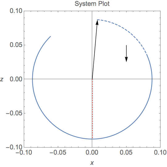
pen1 = {l Sin[\[Theta][t]], -l Cos[\[Theta][t]]} /. sol;
A plot of just the homogenous side. Falls like expected, the down black arrow is the g force
Heres the StateSpaceModel:
model = StateSpaceModel[
    deqns, {{\[Theta][t], \[Pi]}, {\[Theta]'[t], 0}, {\[Omega][t],
      0}, {\[Omega]'[t], 0}}, {u[t], f[t]}, {\[Theta][t]}, t] /.
   rparams /. params
And now the LQR, Q and R matrices :
q = DiagonalMatrix[{1, 100, 100, 0}];
r = 20 {{1}};
gains = Join[
  LQRegulatorGains[{model, 1}, {q, r}], {ConstantArray[0, 4]}]
controlmodel = SystemsModelStateFeedbackConnect[model, gains];
{phi, phidot, omega, omegadot} =
  StateResponse[{controlmodel, {7 \[Pi]/180, 0, 0, 0}}, {0,
    bumpy[t]}, {t, 40}];
And the calculated result:
    86.6683 (-\[Pi] + \[Theta][t]) + 2.23607 \[Omega][t] +
     13.1289 Derivative[1][\[Theta]][t] +
     1.44953 Derivative[1][\[Omega]][t]
After this I went and did a nonlinear system:
nlmodel =
 NonlinearStateSpaceModel[
  deqns, {{\[Theta][t], \[Pi]}, {\[Theta]'[t], 0}, {\[Omega][t],
    0}, {\[Omega]'[t], 0}}, {u[t], f[t]}, {\[Theta][t]}, t]
nlmodeln = nlmodel /. rparams /. params
then a new LQR calculation and plotting the StateResponse
gainsn = Join[
  LQRegulatorGains[{nlmodeln, 1}, {q, r}], {ConstantArray[0, 4]}]
controlmodeln = SystemsModelStateFeedbackConnect[nlmodeln, gains];
{phin, phidotn, omegan, omegadotn} =
 StateResponse[{controlmodeln, {\[Pi], 0, 0, 0}}, {0, bump[t]}, {t,
   40}]
Plot[{phin, omegan}, {t, 0, 11}, PlotRange -> All, ImageSize -> Large,
  PlotTheme -> "Scientific", GridLines -> Automatic,
 PlotLabels -> {\[Theta], \[Omega], \[FormalW]},
 FrameLabel -> {t, A, "Function"}, RotateLabel -> False,
 LabelStyle -> ( FontSize -> 14)]
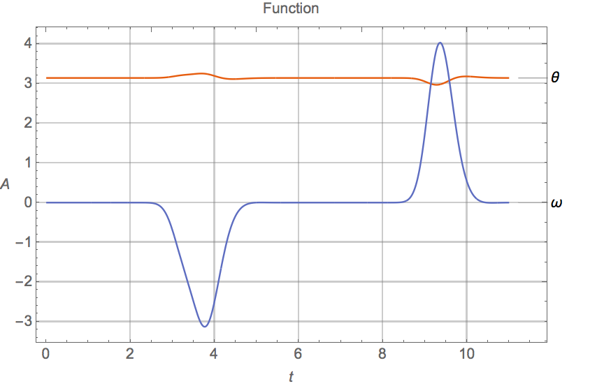
So, As you can see, it's a pretty nice stabilized system. (well, I think so, haha!) Though I couldn't figure out how to plot the input (the control force u[t]) Once I actually programmed this and saw the system trying to react and saw controlforce skyrocket...Well, we're here where we are.
Just to explain some functions and params.
theta is the pendulum body
omega the flywheel angular vel
f[t] is the outside disturbance which is described later as "bump[t]"
bump[t_] :=
 0.2 E^(-10 (t - 3)^2) + 0.4 E^(-10 (t - 3.5)^2) -
  1/2 E^(-10 (t - 9)^2)
and u[t] the control input. At this point, the BLDC motor I have, which is a maxon EC45 Flat, has a maximum RPM of 6200, and an input of (+/-) 2amps, hence the need to restrict the input/control signal to +/- 2.
Thanks for the help/ infos, really appreciate it!


