Message Boards Message Boards

Help needed with code optimization in Manipulate

Posted 11 years ago
I'm trying to build an interactive dynamic presentation with Manipulate about the electric field lines generated by an electric dipole (couple of charges).
In my plan the user should be able to move the two charges generating the field (through a locator) and there would be a third locator for evaluating the field in that point (say point P). Moreover there will be a specific field line passing through that point P.

I've managed to write the code, but it's extremely slow.
The problem seems to be that when I move the point P everything is recalculated within the Manipulate expression, even the field lines, that aren't actually affected by the position of the point P and that requires some time machine for Mathematica's end-front to draw the plot (also because the field lines are set to start/end in a specific - user controlled - set of points around the charges).

So how could I let Mathematica know that only some pieces of code must be re-evaluated when interactively moving some single control (i.e. a locator) and other parts need not?
Browsing the documentation I understand that this should be possible, but it's not easy for me to understand the proper command to use (Hold? Refresh?) and the structure to give to the Manipulate expression.

So if some expert could give me some advice on how to optimize my code to make the presentation much more responsive to the user's interaction I'd be very grateful.

To be more specific here's the (slow) code I've come up with till now. I understand that changing the position of the charges can be slow, as all the field lines should be recalculated, but simply changing the position of the P point should not be so slow as in this case the other field lines needn't be recalculated.
  Manipulate[
   DynamicModule[{xPt, yPt, xq1, yq1, xq2, yq2, r, r1, r2, Emag, Emag1,
     Emag2, Ex, Ex1, Ex2, Ey, Ey1, Ey2, Exx, Eyy,(*qq1,qq2,*)qf,
     VecE, \[Alpha]q, CenterP, FieldPts, EInt}, xPt = startPoint[[1]];
    yPt = startPoint[[2]];
    xq1 = q1pos[[1]];
    yq1 = q1pos[[2]];
    xq2 = q2pos[[1]];
    yq2 = q2pos[[2]];
   (*qq1=SourceCharge1;
   qq2=SourceCharge2;*)r1 = N[Sqrt[(xPt - xq1)^2 + (yPt - yq1)^2], 3];
   r2 = N[Sqrt[(xPt - xq2)^2 + (yPt - yq2)^2], 3];
   Emag1 = qq1/r1^2;
   Emag2 = qq2/r2^2;
   Ex1 = Emag1*(xPt - xq1)/r1;
   Ey1 = Emag1*(yPt - yq1)/r1;
   Ex2 = Emag2*(xPt - xq2)/r2;
   Ey2 = Emag2*(yPt - yq2)/r2;
   Exx = Ex1 + Ex2;
   Eyy = Ey1 + Ey2;
   VecE[x_, y_] :=
    VecE[x, y] = {(qq1 (x - xq1))/((x - xq1)^2 + (y - yq1)^2)^(3/
           2) + (qq2 (x - xq2))/((x - xq2)^2 + (y - yq2)^2)^(3/
           2), (qq1 (y - yq1))/((x - xq1)^2 + (y - yq1)^2)^(3/
           2) + (qq2 (y - yq2))/((x - xq2)^2 + (y - yq2)^2)^(3/2)};
   EInt[x_, y_] :=
    EInt[x, y] = \[Sqrt](((qq1 (x -
                xq1))/((x - xq1)^2 + (y - yq1)^2)^(3/
               2) + (qq2 (x - xq2))/((x - xq2)^2 + (y - yq2)^2)^(3/
               2))^2 + ((qq1 (y - yq1))/((x - xq1)^2 + (y - yq1)^2)^(3/
               2) + (qq2 (y - yq2))/((x - xq2)^2 + (y - yq2)^2)^(3/
               2))^2);
   \[Alpha]q = ArcTan[(yq2 - yq1)/(xq2 - xq1)];
   CenterP = {{(xq1 + xq2)/2, (yq1 + yq2)/2}};
   FieldPts =
    Flatten[{Table[{xq1 + d Cos[\[Alpha] + \[Alpha]q],
        yq1 + d Sin[\[Alpha] + \[Alpha]q]}, {\[Alpha], 0,
        2 \[Pi], \[Pi]/(3 2^s)}],
      Table[{xq2 + d Cos[\[Alpha] + \[Alpha]q],
        yq2 + d Sin[\[Alpha] + \[Alpha]q]}, {\[Alpha], 0,
        2 \[Pi], \[Pi]/(3 2^s) If[qq2 == 0, 2 3 2^s,
          Min[2 \[Pi], Abs[qq1]/Abs[qq2]]]}]}, 1];
   Show[{DensityPlot[
      0.1 + (2/\[Pi] ArcTan[EInt[x, y]])^ExCol, {x, -6 + offset,
       6 - offset}, {y, -6 + offset, 6 - offset},
      ColorFunction -> GrayLevel, ColorFunctionScaling -> False,
      ImageSize -> 800, GridLines -> Automatic,
      BaseStyle -> Directive[Opacity[0.8]],
      Epilog -> {Text[Style[P, 20, RGBColor[0, 0, 0], Bold, Italic],
         startPoint, {0, 1.5}],
        Text[Style[Subscript[q, 1], 24, RGBColor[0, 0, 0], Bold],
         q1pos, {0, 2.5}],
        Text[Style[Subscript[q, 2], 24, RGBColor[0, 0, 0], Bold],
         q2pos, {0, 2.5}],
        Arrowheads[.015], {Dashed, GrayLevel[0.25],
         Line[{{VS*Ex2 + xPt, VS*Ey2 + yPt}, {VS*Exx + xPt,
            VS*Eyy + yPt}}]}, {Dashed, GrayLevel[0.25],
         Line[{{VS*Exx + xPt, VS*Eyy + yPt}, {VS*Ex1 + xPt,
            VS*Ey1 + yPt}}]}, {RGBColor[0, 0.6, 0],
         Disk[q1pos, .25]}, {Blue, Disk[q2pos, .25]}, {Black,
         Disk[startPoint, .1]}, {Thin, RGBColor[0, 0.6, 0],
         Arrow[{startPoint, {VS*Ex1 + xPt, VS*Ey1 + yPt}}]}, {Thin,
         Blue, Arrow[{startPoint, {VS*Ex2 + xPt,
            VS*Ey2 + yPt}}]}, {Thickness[0.0035],
         RGBColor[0.5, 0.1, 0.1],
         Arrow[{startPoint, {VS*Exx + xPt, VS*Eyy + yPt}}]}}],
     If[field,
      StreamPlot[
       VecE[x, y], {x, -6 + offset, 6 - offset}, {y, -6 + offset,
        6 - offset},
       StreamPoints -> {{FieldPts ->
           Directive[Thickness[Tiny], RGBColor[0.9, 0.5, 0.5]], 1},
         Fine, Scaled[1]}, StreamScale -> {0.08, 0.1, 0.0055},
       ImageSize -> 800],
      StreamPlot[{0, 0}, {x, -6 + offset, 6 - offset}, {y, -6 + offset,
         6 - offset}, StreamPoints -> None,
       StreamScale -> {0.08, 0.1, 0.0055}]],
     StreamPlot[
      VecE[x, y], {x, -6 + offset, 6 - offset}, {y, -6 + offset,
       6 - offset},
      StreamPoints -> {{{startPoint, RGBColor[0.5, 0.0, 0.1]}}},
      StreamScale -> 0.05, ImageSize -> 800, GridLines -> Automatic](*,
     StreamScale\[Rule]0.06*)}]], {{startPoint, {-0.4,
     3}}, {-7, -7}, {7, 7},
   Locator}, {{q1pos, {-2, 0}}, {-7, -7}, {7, 7},
   Locator}, {{q2pos, {2, 0}}, {-7, -7}, {7, 7}, Locator},
  Grid[{{Control[{{qq1, 2, "\!\(\*SubscriptBox[\(q\), \(1\)]\)"}, -4,
       4, .5, Appearance -> "Labeled"}],
     Control[{{qq2, -2, "\!\(\*SubscriptBox[\(q\), \(2\)]\)"}, -4,
       4, .5, Appearance -> "Labeled"}]}, {Control[{{d, 0.7,
        "lines start distance form charges"}, 0.1, 4, 0.1,
       Appearance -> "Labeled"}],
     Control[{{s, 1, "lines density"}, 1, 4, 1,
       Appearance -> "Labeled"}]}, {Control[{{VS, 13, "Vector Scale"},
       0, 25, 1, Appearance -> "Labeled"}],
     Control[{{ExCol, 0.3, "Color Scale"}, 0, 1, 0.2,
       Appearance -> "Labeled"}]}, {Control[{{offset, 0,
        "Global range"}, -4, 4, 0.5, Appearance -> "Labeled"}],
     Control[{{field, True, "Show Field lines"}, Checkbox}]}},
  Frame -> All], ControlPlacement -> Top]
Actually, if the code regarding the definition of the field lines starting points:
FieldPts =
  Flatten[{Table[{xq1 + d Cos[\[Alpha] + \[Alpha]q],
      yq1 + d Sin[\[Alpha] + \[Alpha]q]}, {\[Alpha], 0,
      2 \[Pi], \[Pi]/(3 2^s)}],
    Table[{xq2 + d Cos[\[Alpha] + \[Alpha]q],
      yq2 + d Sin[\[Alpha] + \[Alpha]q]}, {\[Alpha], 0,
      2 \[Pi], \[Pi]/(3 2^s) If[qq2 == 0, 2 3 2^s,
        Min[2 \[Pi], Abs[qq1]/Abs[qq2]]]}]}, 1];
is commented out, the presentation becomes much more quick (but the plot will show just the single field lines passing through the point P).
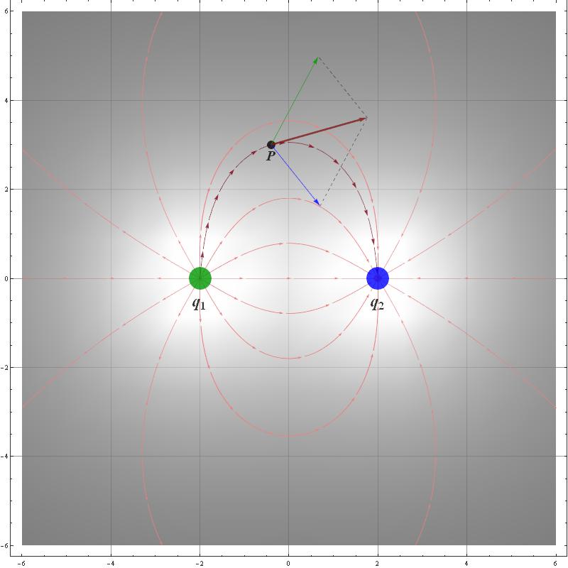
Here is a static image of my WIP presentation:

POSTED BY: Luca M
7 Replies
Why do you need to use DynamicModule inside Manipulate? Most of the slowness when using Dynamics and Manipulate comes down to wrong placement and overuse of  Dynamic Wrapper. Only advice I can give is to keep things simple to be able to debug it. Debugging Dyanmics is not easy. 

Test again each time you add any additional code right away. This way, if things become slow, you know it is in the code just added, and it wil easy to find the problem since you know it is due to the code added.  Add small amount of code, and test right away. Also if you make changes in exisiting code. Test after making any changes, This method always works emoticon. Do not add lots of code and test all later, makes it hard to know where the problem is.
So how could I let Mathematica know that only some pieces of code must be re-evaluated when interactively moving some single control (i.e. a locator) and other parts need not

There are number of ways to do this. see documenation AdvancedManipulateFunctionality
I also wrote some notes on this Here is one Also note at Mathgroup here (which is the method I currently used) also the "Manipulate/Dynamic" section here where-can-i-find-examples-of-good-mathematica-programming-practice has many related and useful links on this subject.

Good luck.
POSTED BY: Nasser M. Abbasi
Hi Luca,

Some simple hints:
  * use the Manipualte option ContinuousAction -> False
  * use the Manipualte option TrackedSymbols :> {myvariable1, mycontrolvariable1, ...}  so that only changes to these variables trigger re-evaluation.  I believe that the default is "Full", i.e. that ALL variables that lexically appear within Manipulate scope, if each/any changes value, it triggers re-eval...you can see how that might really pile up the CPU wait. 

Nasser's pointers contain some good ideas.  As one of them notes, any MathGroup discussion involving John Fultz (of WRI) is bound to be informative about Manipulate and Dynamic functionality. 

I've been meaning for a while to attempt to document my lessons-learned in as nice a way as has Nasser, but in meantime, here are a few points (perhaps some obvious):

* I had previously been under the misapprehension that Manipulate ran its own internal "state machine" a la Nasser's suggested example, but in fact a change to any TrackedSymbol triggers re-evaluating the entire body (1st-argument) of the Manipulate.

* If the body  (1st-argument) of your Manipulate changes the value of a TrackedSymbol,
this will trigger yet another re-evaluation loop.  Of course, unless
such update entails a conditional statement that eventually bypasses
such change, then the re-eval loop will continue forever (or at
least while the visual content is visible on-screen).  

* It does make sense to have Control variables that are NOT TrackedSymbols.  The user can change their state without that triggering a Dynamic update, yet those new state values are "noticed" when other controls or button-pushes subsequently trigger an update. 

* User input on a control variable (e.g. a checkbox) which is NOT a TrackedSymbol can nonetheless trigger updating behavior, if it appears inside an "interior" Dynamic.  Note that it is not the Manipulate body that is re-evaluated but rather the interior Dynamic. 

* Even if a control variable is a TrackedSymbol, if it doesn't appear explicitly (lexically) within the Manipulate body, tickling it won't trigger a body re-evaluation.    (This one is useful to know if one is attempting to wire tricky re-evaluation logic). 

*  Use of a Module[] as a part of the Manipulate body (1st argument) can be useful to isolate calculations on local variables (within the Module) that one does not want  triggering body re-evaluation. 

* A good rule of thumb : if a variable is included in TrackSymbols, it better be localized to within the subject Manipulate, or otherwise it will leak out as a session -global variable (and interfere with same -named variable in another Manipulate instance).   Variables associated with Controls ARE localized.  One means of localizing a variable is to make it a Control variable of type None:  {myvariable, ControlType -> None}
POSTED BY: Frank Iannarilli
Posted 11 years ago
Many thanks to Nasser and Frank Iannarilli for their useful and precious advice.
I've followed their suggestions and I've learned a little bit more. Not enough, though (I know I've still a long way to go...), to find a solution to my problem.

Yet I'm positive that there must be a simple solution for achieving what I want to get.

So I'm asking again for some more concrete advice on how to solve my specific problem, also because it seems I'm too dumb to find the solution by myself even with the help received so far.

In more general terms the problem is rather simple and goes like this (leaving out the code details and the use or not of a Module wrapper that doesn't change much the time response):
Manipulate[
body;    (*here there are some calcs about the field and also the definitions
   graph1=Expression_1;
   graph2=Expression_2;    *)
Show[graph1,graph2],
{{startpoint, {-0.4, 3}}, {-7, -7}, {7, 7}, Locator},
{{q1pos, {-2, 0}}, {-7, -7}, {7, 7}, Locator},
{{q2pos, {2, 0}}, {-7, -7}, {7, 7}, Locator}]
Here the startpoint is the point P in which to calculate (and represent) the field vector and a single field line passing through P (graph1).
q1pos and q2pos are the position of the two charges generating the field and from which start and end more field lines (graph2). Both graphs are generated with Mathematica StreamPlot command.
In my plan, when I move the startpoint, only the graph1 should be dynamically updated (it should be rather fast). I can accept (it's reasonable) that moving the charges q1 and/or q2 and generating all the other field lines can be quite slow (about 1 or 2 seconds' delay).
But if I just change the startpoint position everything is recalculated (also the graph2 that isn't affected by the startpoint position) and the response is slower than it should be.

I've experimented with "ContinuousAction -> False". It improves things but I'd rather have my students have a better dynamical feeling with a continuous action.

I've also tried to use the TrackedSymbols option, but it doesn't seems to solve my problem since all controls ahould be tracked (unless I can use it conditionally with detecting which control is acted upon... is there a way?)

I've also read some of the documentation suggested by Nasser. In particular the Advanced Manipulate Functionality tutorial.
In it I found a possible solution in the section "Using Dynamic inside Manipulate". So I've tried setting
graph1=Dynamic[Expression_1]
but then
Show[graph1,graph2]
doesn't work anymore (I see that there's a long discussion about this in Nasser's links).

The closest I got to the solution I'd like to get is using
graph1=Dynamic[Expression_1]
with
{graph1,graph2}   (*instead of Show[graph1,graph2] *)
This way I get somehow the solution I'm looking for: changing the startpoint position is quick as it doens't trigger a recalculation of the graph2.
But unfortunately, in this way I have two separate graphs as I can't use the Show command to combine them in a single one.

It seems that a bit of more in-depth programming, using conditional statements as in Nasser's "using event driven model with Mathematica Manipulate[] programming", could be the only way to go. But that's a tough solution for me (it will require some more time for me to fully understand and implement it) and, moreover, it's not a simple enough solution that could allow my students to have an intuitive understanding to the code behind the presentation.

If someone is interested to experiment with a real snippet of code (a stripped down version of my previous post) here it is:
 Manipulate[DynamicModule[{VecE, FieldPts, xq1, yq1, xq2, yq2},
   FieldPts = {{-1.3, 0}, {-1.394, 0.35}, {-1.65, 0.606}, {-2.,
      0.7}, {-2.35, 0.606}, {-2.606, 0.35}, {-2.7,
      0}, {-2.606, -0.35}, {-2.35, -0.606}, {-2., -0.7}, {-1.65, \
 -0.606}, {-1.394, -0.35}, {-1.3, 0}, {2.7, 0}, {2.606, 0.35}, {2.35,
      0.606}, {2., 0.7}, {1.65, 0.606}, {1.394, 0.35}, {1.3,
      0}, {1.394, -0.35}, {1.65, -0.606}, {2., -0.7}, {2.35, -0.606}, \
 {2.606, -0.35}, {2.7, 0}}; xq1 = q1pos[[1]];
   yq1 = q1pos[[2]];
  xq2 = q2pos[[1]];
  yq2 = q2pos[[2]];
  VecE[x_,
    y_] := {(2 (x - xq1))/((x - xq1)^2 + (y - yq1)^2)^(
     3/2) + (-2 (x - xq2))/((x - xq2)^2 + (y - yq2)^2)^(3/2), (
     2 (y - yq1))/((x - xq1)^2 + (y - yq1)^2)^(
     3/2) + (-2 (y - yq2))/((x - xq2)^2 + (y - yq2)^2)^(3/2)};
  graph1 =
   StreamPlot[VecE[x, y], {x, -6, 6}, {y, -6, 6},
    StreamPoints -> {{{startPoint, RGBColor[0.5, 0.0, 0.1]}}},
    StreamScale -> 0.05, GridLines -> Automatic, ImageSize -> 600];
  graph2 =
   StreamPlot[VecE[x, y], {x, -6, 6}, {y, -6, 6},
    StreamPoints -> {{FieldPts ->
        Directive[Thickness[Tiny], RGBColor[0.9, 0.5, 0.5]], 1},
      Fine, Scaled[1]}, StreamScale -> {0.08, 0.1, 0.0055},
    GridLines -> Automatic, ImageSize -> 600];
  Show[{graph1, graph2}]],
{{startPoint, {-0.4, 3}}, {-7, -7}, {7, 7},
  Locator}, {{q1pos, {-2, 0}}, {-7, -7}, {7, 7},
  Locator}, {{q2pos, {2, 0}}, {-7, -7}, {7, 7}, Locator}]

Thanks in advance for your help.

Luca
POSTED BY: Luca M
Hi Luca,

Here is a bit of progress, at least to make the field-lines option snappy. 
  Changes: 
    Replace DynamicModule with Module. 
    add in graphics holder variables g1,g2on,g2off, g3 and their ControlType->None declarations (they are external variables w.r.t. Module) 
    Make Dynamic[If[field,Show[{g1,g2on,g3}],Show[{g1,g2off,g3}]]] what is returned by the Module
  Manipulate[
   Module[{xPt, yPt, xq1, yq1, xq2, yq2, r, r1, r2, Emag, Emag1, Emag2,
     Ex, Ex1, Ex2, Ey, Ey1, Ey2, Exx, Eyy,(*qq1,qq2,*)qf,
     VecE, \[Alpha]q, CenterP, FieldPts, EInt},
    xPt = startPoint[[1]];
    yPt = startPoint[[2]];
    xq1 = q1pos[[1]];
    yq1 = q1pos[[2]];
    xq2 = q2pos[[1]];
   yq2 = q2pos[[2]];
   (*qq1=SourceCharge1;
   qq2=SourceCharge2;*)r1 = N[Sqrt[(xPt - xq1)^2 + (yPt - yq1)^2], 3];
   r2 = N[Sqrt[(xPt - xq2)^2 + (yPt - yq2)^2], 3];
   Emag1 = qq1/r1^2;
   Emag2 = qq2/r2^2;
   Ex1 = Emag1*(xPt - xq1)/r1;
   Ey1 = Emag1*(yPt - yq1)/r1;
   Ex2 = Emag2*(xPt - xq2)/r2;
   Ey2 = Emag2*(yPt - yq2)/r2;
   Exx = Ex1 + Ex2;
   Eyy = Ey1 + Ey2;
   VecE[x_, y_] :=
    VecE[x, y] = {(qq1 (x - xq1))/((x - xq1)^2 + (y - yq1)^2)^(3/
           2) + (qq2 (x - xq2))/((x - xq2)^2 + (y - yq2)^2)^(3/
           2), (qq1 (y - yq1))/((x - xq1)^2 + (y - yq1)^2)^(3/
           2) + (qq2 (y - yq2))/((x - xq2)^2 + (y - yq2)^2)^(3/2)};
   EInt[x_, y_] :=
    EInt[x, y] = \[Sqrt](((qq1 (x -
                xq1))/((x - xq1)^2 + (y - yq1)^2)^(3/
               2) + (qq2 (x - xq2))/((x - xq2)^2 + (y - yq2)^2)^(3/
               2))^2 + ((qq1 (y - yq1))/((x - xq1)^2 + (y - yq1)^2)^(3/
               2) + (qq2 (y - yq2))/((x - xq2)^2 + (y - yq2)^2)^(3/
               2))^2);
   \[Alpha]q = ArcTan[(yq2 - yq1)/(xq2 - xq1)];
   CenterP = {{(xq1 + xq2)/2, (yq1 + yq2)/2}};
   FieldPts =
    Flatten[{Table[{xq1 + d Cos[\[Alpha] + \[Alpha]q],
        yq1 + d Sin[\[Alpha] + \[Alpha]q]}, {\[Alpha], 0,
        2 \[Pi], \[Pi]/(3 2^s)}],
      Table[{xq2 + d Cos[\[Alpha] + \[Alpha]q],
        yq2 + d Sin[\[Alpha] + \[Alpha]q]}, {\[Alpha], 0,
        2 \[Pi], \[Pi]/(3 2^s) If[qq2 == 0, 2 3 2^s,
          Min[2 \[Pi], Abs[qq1]/Abs[qq2]]]}]}, 1];
   g1 = DensityPlot[
     0.1 + (2/\[Pi] ArcTan[EInt[x, y]])^ExCol, {x, -6 + offset,
      6 - offset}, {y, -6 + offset, 6 - offset},
     ColorFunction -> GrayLevel, ColorFunctionScaling -> False,
     ImageSize -> 800, GridLines -> Automatic,
     BaseStyle -> Directive[Opacity[0.8]],
     Epilog -> {Text[Style[P, 20, RGBColor[0, 0, 0], Bold, Italic],
        startPoint, {0, 1.5}],
       Text[Style[Subscript[q, 1], 24, RGBColor[0, 0, 0], Bold],
        q1pos, {0, 2.5}],
       Text[Style[Subscript[q, 2], 24, RGBColor[0, 0, 0], Bold],
        q2pos, {0, 2.5}],
       Arrowheads[.015], {Dashed, GrayLevel[0.25],
        Line[{{VS*Ex2 + xPt, VS*Ey2 + yPt}, {VS*Exx + xPt,
           VS*Eyy + yPt}}]}, {Dashed, GrayLevel[0.25],
        Line[{{VS*Exx + xPt, VS*Eyy + yPt}, {VS*Ex1 + xPt,
           VS*Ey1 + yPt}}]}, {RGBColor[0, 0.6, 0],
        Disk[q1pos, .25]}, {Blue, Disk[q2pos, .25]}, {Black,
        Disk[startPoint, .1]}, {Thin, RGBColor[0, 0.6, 0],
        Arrow[{startPoint, {VS*Ex1 + xPt, VS*Ey1 + yPt}}]}, {Thin,
        Blue, Arrow[{startPoint, {VS*Ex2 + xPt,
           VS*Ey2 + yPt}}]}, {Thickness[0.0035],
        RGBColor[0.5, 0.1, 0.1],
        Arrow[{startPoint, {VS*Exx + xPt, VS*Eyy + yPt}}]}}];
   g2on =
    StreamPlot[
     VecE[x, y], {x, -6 + offset, 6 - offset}, {y, -6 + offset,
      6 - offset},
     StreamPoints -> {{FieldPts ->
         Directive[Thickness[Tiny], RGBColor[0.9, 0.5, 0.5]], 1}, Fine,
        Scaled[1]}, StreamScale -> {0.08, 0.1, 0.0055},
     ImageSize -> 800];
   g2off = StreamPlot[{0, 0}, {x, -6 + offset,
      6 - offset}, {y, -6 + offset, 6 - offset}, StreamPoints -> None,
     StreamScale -> {0.08, 0.1, 0.0055}];
   g3 = StreamPlot[
     VecE[x, y], {x, -6 + offset, 6 - offset}, {y, -6 + offset,
      6 - offset},
     StreamPoints -> {{{startPoint, RGBColor[0.5, 0.0, 0.1]}}},
     StreamScale -> 0.05, ImageSize -> 800, GridLines -> Automatic](*,
   StreamScale\[Rule]0.06*);
   Dynamic[If[field, Show[{g1, g2on, g3}], Show[{g1, g2off, g3}]]]],
  {{startPoint, {-0.4, 3}}, {-7, -7}, {7, 7}, Locator},
  {{q1pos, {-2, 0}}, {-7, -7}, {7, 7}, Locator},
  {{q2pos, {2, 0}}, {-7, -7}, {7, 7}, Locator},
  {g1, ControlType -> None},
  {g2on, ControlType -> None},
  {g2off, ControlType -> None},
  {g3, ControlType -> None},
  Grid[{{Control[{{qq1, 2, "\!\(\*SubscriptBox[\(q\), \(1\)]\)"}, -4,
       4, .5, Appearance -> "Labeled"}],
     Control[{{qq2, -2, "\!\(\*SubscriptBox[\(q\), \(2\)]\)"}, -4,
       4, .5, Appearance -> "Labeled"}]}, {Control[{{d, 0.7,
        "lines start distance form charges"}, 0.1, 4, 0.1,
       Appearance -> "Labeled"}],
     Control[{{s, 1, "lines density"}, 1, 4, 1,
      Appearance -> "Labeled"}]}, {Control[{{VS, 13, "Vector Scale"},
      0, 25, 1, Appearance -> "Labeled"}],
    Control[{{ExCol, 0.3, "Color Scale"}, 0, 1, 0.2,
      Appearance -> "Labeled"}]}, {Control[{{offset, 0,
       "Global range"}, -4, 4, 0.5, Appearance -> "Labeled"}],
    Control[{{field, True, "Show Field lines"}, Checkbox}]}},
  Frame -> All], ControlPlacement -> Top]
POSTED BY: Frank Iannarilli
Posted 11 years ago
Thanks Frank!

I think your version mark a great step forward in the code speed optimization. I've tried it (and I'll study it later with some ease) and I can say that now the time response is much shorter and almost acceptable (practically).

Anyway I must say that the core (theorical) problem seems not yet solved.

That is, when I move the startPoint locator the overall field lines are still recalculated (and they shouldn't be). Even if the time response is almost acceptable now (with your changes) I'm afraid the presentation could be rather slow with a higher number of field lines set or with an older and much slower machine (as one you could find in public schools),

Anyway you gave me a great help and headway and I thank you very much for your time and for the remarkable improvements/optimization you made on my initial code.
POSTED BY: Luca M
Hi again Luca,

Here's another cut that just about solves the "core" problem. 
   Here's what's new and going on:

* Now using Manipulate's Initialization option to define epiPFunc[], which contains the components of the Epilog to the DensityPlot (g1) that only vary with your point P.  It's necessary (AFAIK) to remove this code from the large Module that forms most of the Manipulate body so that its execution doesn't also spur the (unnecessary) execution of the Module's contents. 

* Coupled with this separation of Epilog into two parts, is the enclosure of the Epilog's argument within a Dynamic[], i.e. we now have a so-called "interior" Dynamic within a Manipulate -- this trick is discussed in the documentation tutorial "Advanced Manipulate Functionality" ("using Dynamic inside Manipulate").  This allows updates to point P (locator) to trigger updates to the Epilog without incurring the updates to the DensityPlot field, which unnecessary when only P is changing. 

* I pulled the Dynamic[Show[{g1, If[field, g2on, g2off], g3}]] outside of the large Module and simplified it a bit.  It seems that the way Show must combine the graphics is such that it all should be wrapped up within Dynamic.  Merely surrounding the If[] statement with Dynamic doesn't work.  

* I tried to speed up the g3 graphic (streamline through P) in response to changes of point P, but I believe this graphic is fundamentally slow.  You can see my attempts here in my relocating your VecE[] function from the large Module to the Initialization section.  So to short-circuit things while leaving the code structure in place, within the g3 StreamPlot, I replaced the startPoint argument with q2pos.  You can see that I tried to enclose its StreamPoints option with a Dynamic[], but this doesn't help the fundamental slowness.  So for now, the g3 streamline through P is not displayed (it goes through q2!) 


  Manipulate[
   Module[{xq1, yq1, xq2, yq2,(*qq1,qq2,*)qf, \[Alpha]q, CenterP,
     FieldPts, EInt},
    (*qq1=SourceCharge1;
    qq2=SourceCharge2;*)
    xq1 = q1pos[[1]];
    yq1 = q1pos[[2]];
    xq2 = q2pos[[1]];
    yq2 = q2pos[[2]];
   EInt[x_, y_] :=
    EInt[x, y] = \[Sqrt](((qq1 (x -
                xq1))/((x - xq1)^2 + (y - yq1)^2)^(3/
               2) + (qq2 (x - xq2))/((x - xq2)^2 + (y - yq2)^2)^(3/
               2))^2 + ((qq1 (y - yq1))/((x - xq1)^2 + (y - yq1)^2)^(3/
               2) + (qq2 (y - yq2))/((x - xq2)^2 + (y - yq2)^2)^(3/
               2))^2);
   \[Alpha]q = ArcTan[(yq2 - yq1)/(xq2 - xq1)];
   CenterP = {{(xq1 + xq2)/2, (yq1 + yq2)/2}};
   FieldPts =
    Flatten[{Table[{xq1 + d Cos[\[Alpha] + \[Alpha]q],
        yq1 + d Sin[\[Alpha] + \[Alpha]q]}, {\[Alpha], 0,
        2 \[Pi], \[Pi]/(3 2^s)}],
      Table[{xq2 + d Cos[\[Alpha] + \[Alpha]q],
        yq2 + d Sin[\[Alpha] + \[Alpha]q]}, {\[Alpha], 0,
        2 \[Pi], \[Pi]/(3 2^s) If[qq2 == 0, 2 3 2^s,
          Min[2 \[Pi], Abs[qq1]/Abs[qq2]]]}]}, 1];
   g1 = DensityPlot[
     0.1 + (2/\[Pi] ArcTan[EInt[x, y]])^ExCol, {x, -6 + offset,
      6 - offset}, {y, -6 + offset, 6 - offset},
     ColorFunction -> GrayLevel, ColorFunctionScaling -> False,
     ImageSize -> 800, GridLines -> Automatic,
     BaseStyle -> Directive[Opacity[0.8]],
     Epilog ->
      Dynamic[Join[{Text[
          Style[Subscript[q, 1], 24, RGBColor[0, 0, 0], Bold],
          q1pos, {0, 2.5}],
         Text[Style[Subscript[q, 2], 24, RGBColor[0, 0, 0], Bold],
          q2pos, {0, 2.5}],
         Arrowheads[.015], {RGBColor[0, 0.6, 0],
          Disk[q1pos, .25]}, {Blue, Disk[q2pos, .25]}}, epiPFunc[]]]];
   g2on =
    StreamPlot[
     VecE[x, y], {x, -6 + offset, 6 - offset}, {y, -6 + offset,
      6 - offset},
     StreamPoints -> {{FieldPts ->
         Directive[Thickness[Tiny], RGBColor[0.9, 0.5, 0.5]], 1}, Fine,
        Scaled[1]}, StreamScale -> {0.08, 0.1, 0.0055},
     ImageSize -> 800];
   g2off = StreamPlot[{0, 0}, {x, -6 + offset,
      6 - offset}, {y, -6 + offset, 6 - offset}, StreamPoints -> None,
     StreamScale -> {0.08, 0.1, 0.0055}];
   g3 = StreamPlot[
     VecE[x, y], {x, -6 + offset, 6 - offset}, {y, -6 + offset,
      6 - offset},
     StreamPoints -> Dynamic[{{{q2pos, RGBColor[0.5, 0.0, 0.1]}}}],
     StreamScale -> 0.05, ImageSize -> 800, GridLines -> Automatic(*,
     StreamScale\[Rule]0.06*)]
   ];
  Dynamic[Show[{g1, If[field, g2on, g2off], g3}]],
  {{startPoint, {-0.4, 3}}, {-7, -7}, {7, 7}, Locator},
  {{q1pos, {-2, 0}}, {-7, -7}, {7, 7}, Locator},
  {{q2pos, {2, 0}}, {-7, -7}, {7, 7}, Locator},
  {g1, ControlType -> None},
  {g2on, ControlType -> None},
  {g2off, ControlType -> None},
  {g3, ControlType -> None},
  Grid[{{Control[{{qq1, 2, "\!\(\*SubscriptBox[\(q\), \(1\)]\)"}, -4,
       4, .5, Appearance -> "Labeled"}],
     Control[{{qq2, -2, "\!\(\*SubscriptBox[\(q\), \(2\)]\)"}, -4,
       4, .5, Appearance -> "Labeled"}]}, {Control[{{d, 0.7,
        "lines start distance form charges"}, 0.1, 4, 0.1,
       Appearance -> "Labeled"}],
     Control[{{s, 1, "lines density"}, 1, 4, 1,
       Appearance -> "Labeled"}]}, {Control[{{VS, 13, "Vector Scale"},
       0, 25, 1, Appearance -> "Labeled"}],
     Control[{{ExCol, 0.3, "Color Scale"}, 0, 1, 0.2,
       Appearance -> "Labeled"}]}, {Control[{{offset, 0,
        "Global range"}, -4, 4, 0.5, Appearance -> "Labeled"}],
     Control[{{field, True, "Show Field lines"}, Checkbox}]}},
   Frame -> All], ControlPlacement -> Top,
  Initialization :> {VecE[x_, y_] :=
     VecE[x, y] = Module[{xq1, yq1, xq2, yq2},
       xq1 = q1pos[[1]];
       yq1 = q1pos[[2]];
       xq2 = q2pos[[1]];
       yq2 = q2pos[[2]];
       {(qq1 (x - xq1))/((x - xq1)^2 + (y - yq1)^2)^(3/
             2) + (qq2 (x - xq2))/((x - xq2)^2 + (y - yq2)^2)^(3/
             2), (qq1 (y - yq1))/((x - xq1)^2 + (y - yq1)^2)^(3/
             2) + (qq2 (y - yq2))/((x - xq2)^2 + (y - yq2)^2)^(3/2)}],
   
    epiPFunc[] :=
     Module[{xq1, yq1, xq2, yq2, xPt, yPt, r, r1, r2, Emag, Emag1,
       Emag2, Ex, Ex1, Ex2, Ey, Ey1, Ey2, Exx, Eyy},
      xPt = startPoint[[1]];
      yPt = startPoint[[2]];
      xq1 = q1pos[[1]];
      yq1 = q1pos[[2]];
      xq2 = q2pos[[1]];
     yq2 = q2pos[[2]];
     r1 = N[Sqrt[(xPt - xq1)^2 + (yPt - yq1)^2], 3];
     r2 = N[Sqrt[(xPt - xq2)^2 + (yPt - yq2)^2], 3];
     Emag1 = qq1/r1^2;
     Emag2 = qq2/r2^2;
     Ex1 = Emag1*(xPt - xq1)/r1;
     Ey1 = Emag1*(yPt - yq1)/r1;
     Ex2 = Emag2*(xPt - xq2)/r2;
     Ey2 = Emag2*(yPt - yq2)/r2;
     Exx = Ex1 + Ex2;
     Eyy = Ey1 + Ey2;
     Return[{Text[Style[P, 20, RGBColor[0, 0, 0], Bold, Italic],
        startPoint, {0, 1.5}],
       Arrowheads[.015], {Dashed, GrayLevel[0.25],
        Line[{{VS*Ex2 + xPt, VS*Ey2 + yPt}, {VS*Exx + xPt,
           VS*Eyy + yPt}}]}, {Dashed, GrayLevel[0.25],
        Line[{{VS*Exx + xPt, VS*Eyy + yPt}, {VS*Ex1 + xPt,
           VS*Ey1 + yPt}}]}, {Black, Disk[startPoint, .1]}, {Thin,
        RGBColor[0, 0.6, 0],
        Arrow[{startPoint, {VS*Ex1 + xPt, VS*Ey1 + yPt}}]}, {Thin,
        Blue,
        Arrow[{startPoint, {VS*Ex2 + xPt,
           VS*Ey2 + yPt}}]}, {Thickness[0.0035],
        RGBColor[0.5, 0.1, 0.1],
        Arrow[{startPoint, {VS*Exx + xPt, VS*Eyy + yPt}}]}}];
     ]}]
POSTED BY: Frank Iannarilli
Posted 11 years ago
Thanks again Frank

Anyway I think we're in a "cul-de-sac".
With your last solution moving the startPoint doesn't affect anymore the g3 graph (nor the other graphs) and so the Dynamic[Show[...]] is not re-evaluated (your code proves that). But this way the g3 graphs loses its meaning.

I think that there's no way out or a possible solution with using a Show command to combine the plots. Everytime some control changes one of the graphs, all the Show content will be re-evaluated. Only way out would be if the Show could combine a graph wrapped with Dynamic with other ones. But that's not possible with Show.

So I think that, if there's a solution to the "dipole" presentation problem (and I'm beginning to think there's not one with this approach), then the graphs should be combined with some alternative way and not with a Show command.
Maybe using the Prolog/Epilog/Inset applied to a single StreamPlot is the right way (I don't know much about those options so I'll need some time to experiment).

So I'm thinking about starting again from scratch and trying to build a static single graph combining the three graphs with the Prolog/Epilog/Inset options. Then I'll try to make it interactive and will think about placing the appropriate Dynamic wrappers.
POSTED BY: Luca M
Reply to this discussion
Community posts can be styled and formatted using the Markdown syntax.
Reply Preview
Attachments
Remove
or Discard

Group Abstract Group Abstract