Hope it was helpful.

There is a different interpretation between the $R^2$ calculated using LinearModelFit and NonlinearModel but not because of something intrinsically different between linear and nonlinear models but rather that Mathematica chooses to use two different formulas for $R^2$ for the two procedures.

LinearModelFit uses $1-{{SS_{res}}\over{SS_{corrected Total}}}$ and NonlinearModelFit uses $1-{{SS_{res}}\over{SS_{uncorrected Total}}}$. One can see this by fitting the same linear model in LinearModelFit and NonlinearModelFit.

(I have no doubt you read somewhere there there's a difference in meaning in adjusted R2 for linear and nonlinear models. The formula for adjusted R2 only depends on the number of predictor variables. Maybe you're remembering that R2 (adjusted or not) can be more than misleading when the intercept is forced through zero.?)

You don't have to frame everything as a hypothesis test. Getting the standard error of prediction for the mean or of a single new prediction might be a good summary statistic. If the resulting NonlinearModelFit output is stored in nlm. then

nlm["EstimatedVariance"]^0.5

gives you the estimate of the standard error of estimate.

You have to ask yourself (as someone knowing the subject matter) "Is that standard error small enough to satisfy my objectives?" That is a subject matter decision and NOT a statistical decision.

95% Confidence bands for the mean prediction or 95% prediction intervals for an individual prediction are found respectively with

nlm["MeanPredictionBands"]
nlm["SinglePredictionBands"]

You can look at the residuals to check for deviations from the assumptions such as a common variability about the curve and if the pattern of residuals appears to be just a "cloud of points" rather than say the observations in the middle having mostly positive residuals and the extreme lower or upper observations having negative residuals indicating a lack-of-fit.

I've not yet answered your direct question about "testing whether the fit is good". One can perform a test of statistical significance by using the information in the ANOVATable. Again, if the results of NonlinearModelFit are stored in nlm, then

nlm["ANOVATable"]

gets you something like

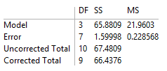
You can grab the information in that table to obtain a P-value for the fit (smaller P-values are associated with better fits than just using the mean of the response variable):

anova = nlm["ANOVATableEntries"]
(* {{3, 65.8809, 21.9603}, {7, 1.59998, 0.228568}, {10, 67.4809}, {9, 66.4376}} *)

fRatio = anova[[1, 3]]/anova[[2, 3]]
(* 96.0777 *) 

pValue = 1 -  CDF[FRatioDistribution[anova[[1, 1]], anova[[2, 1]]], fRatio]
(* 4.73418*10^-6 *)

What question do you want associated with a test of significance? Is it about specific parameters? Linear combinations of parameters? Predictions? NonlinearModelFit can certainly perform the appropriate test or provide information to be able to construct an appropriate test. One just needs to be specific about what you want to test and under what conditions.

Tests of significance aren't necessarily very useful unless you have some idea as to what kind of difference from a hypothesized value you're looking for. Maybe estimation rather than hypothesis testing is what might be more appropriate for your needs.

Also, "the probability of getting such a fit by chance is p" is not quite right about resulting P-values. A P-value is the probability of observing a test statistic at least as extreme as what you observed when a specified null hypothesis about the value of some unknown quantity is true.