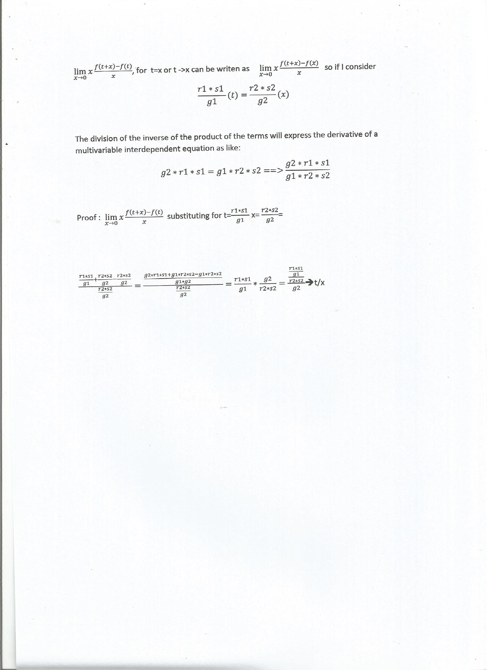
When we consider multivariable derivatives related to same variable with different values, there can be a simplification of the manner to calculate a derivative that gives rise to the possibility to calculate by other means the la grangian point at which the total volume mass time expression between two celestial bodies equals , a point at which the distance gives rise to a certain value that express the limit of the derivative to zero and that is equivalent to a distance between the bodies where the value of gravity time multiple is equal meaning that the bodie is pulled in equal terms of proportion.

r1= RandomReal[6471000,{200}]  radius of earth in meters
r2=RandomReal[695510000,{200}] radius of the sun in meters
s=RandomReal[149600000000,{200}] distance from the sun in meters
g1=RandomReal[9.86,{200}] gravity of earth
g2=RandomReal[274,{200}] gravity of sun
s2=(g2*r1*s)/(2*r2*g1) interrelated equation to obtain an intermediate distance from earth to the sun
s1=s-s2
a=(r1*s1)/g1  total space mass time relation to earth
b=(r2*s2)/g2  total space mass time relation to sun; both equals each other at a given distance
y=(g2*r1*s1)/(g1*r2*s2) third variable obtained from a rule of proportion that equals the aplication of the theorem for the limit of a derivative
ListPlot[a]
ListPlot[b]
ListPolarPlot[s2]
ListPolarPlot[y]
data=Table[Mod[s2,y],{s2,0,Pi,Pi},{y,0,Pi,Pi}]
ListPlot[data,InterpolationOrder->3, ColorFunction->{s2->Yellow,y->Blue,s1->Green}]
ContourPlot3D[Sin[s2*s1/y] ,{s2,-Pi,Pi},{s1,-Pi,Pi},{y,-Pi,Pi}]
Run the program and notice that the simple proportion between two analogus functions alows to obtain a third variable that is related to the applied principle of limit of a derivative. Notice that a and b have equal values for a certain distance from the sun and from earth expressed in space per mass per second. the distance at this point makes the bodie there located to be in the same relative position.
r1= RandomReal[6471000,{200}]
r2=RandomReal[695510000,{200}]
s=RandomReal[149600000000,{200}]
g1=RandomReal[9.86,{200}]
g2=RandomReal[274,{200}]
s2=(g2*r1*s)/(2*r2*g1)
s1=s-s2
a=(r1*s1)/g1
b=(r2*s2)/g2
y=(g2*r1*s1)/(g1*r2*s2)
ListPlot[a]
ListPlot[b]
ListPolarPlot[s2]
ListPolarPlot[y]
data=Table[Mod[s2,y],{s2,0,Pi,Pi},{y,0,Pi,Pi}]
ListPlot[data,InterpolationOrder->3, ColorFunction->{s2->Yellow,y->Blue,s1->Green}]
ContourPlot3D[Sin[s2*s1/y] ,{s2,-Pi,Pi},{s1,-Pi,Pi},{y,-Pi,Pi}]
tahnk you , feel free to aply the rule to any other object distance gravity related condition: black holes for instance.
 Attachments: