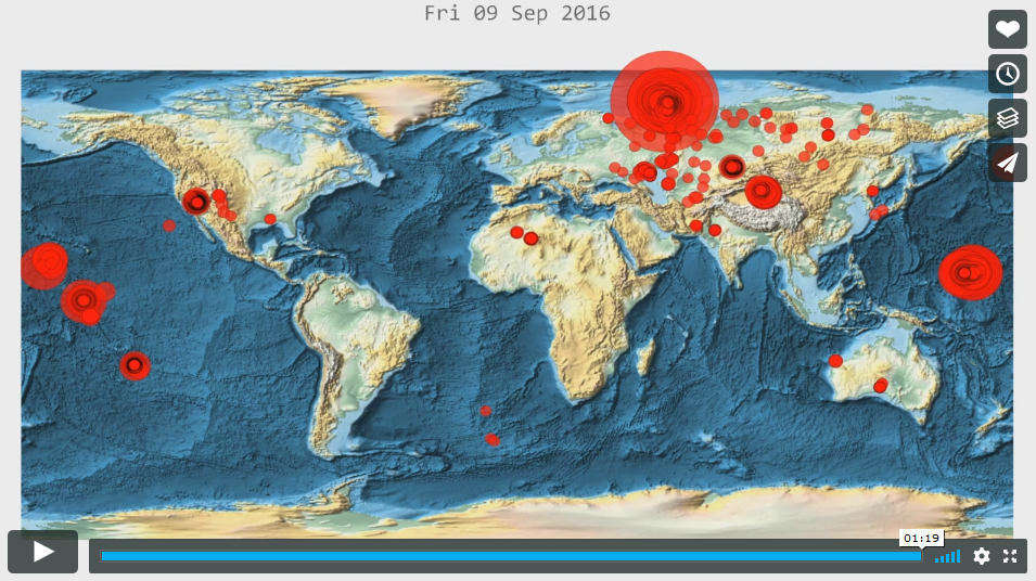
A couple weeks ago, I spent the evening falling down a rabbit hole, reading about the largest nuclear bombs detonated by humans. As usual, this made me wonder if I could do anything related to this topic in the Wolfram Language. After reading about the effects of the largest nuclear bomb and the radius these effects were measured or observed from, I found that GeoGraphics came in quite handy.
On Oct 30, 1961, the worlds largest nuclear bomb ever ever used was detonated by the Soviet Union, above the arctic circle. The yield of this device, known as Tsar Bomba, was approximately 58 megatons.
In[4]:= Entity["NuclearExplosion",
  "UnionSovietSocialistRepublics10301961Test2"]["Yield"]

Out[4]= Quantity[5.8*10^4, "KilotonsOfTNT"]
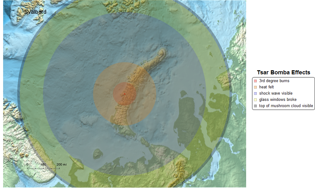
The device was a "hydrogen bomb" which is a device that uses a fission explosion to compress a sample of hydrogen to produce a more powerful thermonuclear fusion explosion. A larger 100 Megaton device was built, but never detonated due to concerns of radioactive fallout to populated areas and the inability of the pilots to escape the site in time. As it stands, the Tsar Bomba explosion barely allowed the pilots to escape as their plane dropped 1 km due to the shock wave, but the pilots were able to recover and land safely. The following shows a set of concentric disks showing the extent of various effects of this explosion.
In[5]:= tsar = GeoPosition[{73.8072, 54.98167`}];

In[6]:= legend = Labeled[
   SwatchLegend[{Directive[Red, Opacity[.3]], Directive[Orange, Opacity[.3]],
     Directive[Blue, Opacity[.2]], Directive[Yellow, Opacity[.2]],
     Directive[Black, Opacity[.3]]}, {"3rd degree burns", "heat felt",
     "shock wave visible", "glass windows broke",
     "top of mushroom cloud visible"}, LegendFunction -> "Frame"],
   Text[Style["Tsar Bomba Effects", Bold, 18]], Top];

In[8]:= text = {Text[Style["Moscow", 12],
    Entity["City", {"Moscow", "Moscow", "Russia"}], {0, 1}],
   Text[Style["St. Petersburg", 12],
    Entity["City", {"SaintPetersburg", "SaintPetersburg", "Russia"}], {0, 1}],
    Text[Style["Greenland", 18], Entity["Country", "Greenland"]],
   Text[Style["Sweden", 18], Entity["Country", "Sweden"]],
   Text[Style["Svalbard", 18], Entity["Country", "Svalbard"]], White,
   Text[Style["+", 36], GeoPosition[{90, 0}]]};

In[9]:= map[km_] := Grid[{
   {
    GeoGraphics[{
      GeoStyling[Opacity[.3]], Red, PointSize[.007],
      Point[Entity["City", {"Moscow", "Moscow", "Russia"}]],
      Point[Entity["City", {"SaintPetersburg", "SaintPetersburg", "Russia"}]],
      Point[tsar], GeoDisk[tsar, Quantity[100, "Kilometers"]],
      Black, text,
      GeoVisibleRegion[
       GeoPosition[{73.80722222222222`, 54.98166666666667`, 67000}]],
      Orange, GeoDisk[tsar, Quantity[270, "Kilometers"]],
      GeoStyling[Opacity[.2]], Blue,
      GeoDisk[tsar, Quantity[700, "Kilometers"]],
      Yellow, GeoDisk[tsar, Quantity[900, "Kilometers"]]},
     GeoGridRange -> {{-1.3, 1.3}, {-1, 1}} km/4000,
     GeoBackground -> "ReliefMap", ImageSize -> {800, 600},
     GeoProjection -> "Orthographic", GeoCenter -> tsar,
     GeoScaleBar -> "Miles", GeoZoomLevel -> 5], legend}
   }
  ]

In[11]:= map[500]
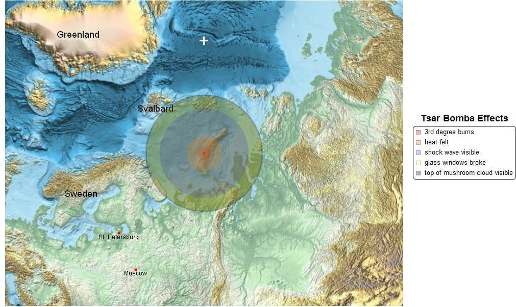
We can zoom out a bit to get a better idea how far this was from various landmarks.
map[1500]
I went on to explore the location, date, and yield of other nuclear explosions around the world and created an animation showing 1 explosion per frame. First, I used EntityValue to obtain the data for all available explosions.
nuc = EntityValue["NuclearExplosion", {"Entity", "Date", "Yield"}];
Then I selected only those with all the necessary data populated and sorted them by date.
In[15]:= clean = Select[nuc, FreeQ[#, _Missing] &];

In[16]:= sorted = SortBy[clean, JulianDate[#[[2]]] &];

In[17]:= sorted // Length

Out[17]= 1913
For scaling purposes, I needed to define the largest one.
In[18]:= max = {#[[2]], Rule[#[[1]], #[[3]]]} &@SortBy[sorted, #[[3]] &][[-1]]

Out[18]= {DateObject[{1961, 10, 30, 8, 33, 27.}, "Instant", "Gregorian", 0.],
 Entity["NuclearExplosion", "UnionSovietSocialistRepublics10301961Test2"] ->
  Quantity[5.8*10^4, "KilotonsOfTNT"]}

In[19]:= rules = {#[[2]], Rule[#[[1]], #[[3]]]} & /@ sorted;
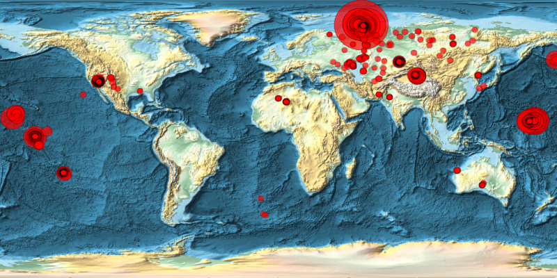
I used GeoBubbleChart to plot all of the explosions with the size of the bubble proportional to it's yield. Many of the explosions happened near each other in various testing areas so you have lots of overlapping bubbles.
In[24]:= GeoBubbleChart[{rules[[1 ;; length]][[All, 2]], {max[[2]]}}, ImageSize -> 800,
  GeoZoomLevel -> 2, GeoBackground -> "ReliefMap", GeoRange -> All,
 ChartElements -> {Automatic, None}, ChartStyle -> {Red}]
An animation running from 1945 all the way up to 2017 can be generated with the following program.
Do[
 Export["Frame" <>
   ToString[
    PaddedForm[i - 1, 4, NumberPadding -> "0",
     NumberSigns -> {"", ""}]] <> ".png",
  GeoBubbleChart[{rules[[1 ;; i]][[All, 2]], {max[[2]]}},
   ImageSize -> {1920, 1080}, GeoZoomLevel -> 2,
   GeoBackground -> "ReliefMap", GeoRange -> All,
   ChartElements -> {Automatic, None}, ChartStyle -> {Red},
   PlotLabel ->
    Style[DateString[
      rules[[i, 1]], {"DayNameShort", " ", "Day", " ",
       "MonthNameShort", " ", "Year"}], {FontFamily -> "Consolas",
      FontSize -> 42}]]],
 {i, 1, length, 1}]
