Introduction
A couple of days ago on 1 July The Economist tweeted this:
Since he was elected in 2016 Donald Trump has made 1,384 mentions of foreign countries on Twitter. Can you guess which one he named most often?
It claims that in spite of the "special relationship" with the UK, it is only ranked 15th of the countries and territories tweeted about. It also says that Puerto Rico, Mexico and China are in fifth, fourth and third places respectively (countries and territories). According to The Economist North Korea is ranked in second place with 163 mentions.
A couple of years ago I read the excellent book "A Mathematician Reads the Newspaper" by John Allen Paulos; and I wonder how much of the daily news coverage can we check using the Wolfram Language. In a future post I will speak about another project that we are doing with several members of this community that goes in a similar direction. We call it "computational conversations". With a bit of luck you might hear about it at the Wolfram Technology Conference later this year.
Initial analysis ----------
It turns out that I have been monitoring @realDonaldTrump's tweets using IFTTT since early 2017. I attach excel files to this post. To have a look at the first tweet we first set the directory and load the raw data files:
SetDirectory[NotebookDirectory[]]
dataraw = Import /@ FileNames["Trump*.xlsx"];
As the first file (without a number) will be read in last (alphabetical order), this is the first tweet data:
dataraw[[5, 1, 1]] // TableForm

It is from January 26th, 2017, a couple of days after his inauguration.
In oder to figure out which countries Mr Trump talks about we use the function TextCases, a recently updated function:
tweettexts = Join[dataraw[[1, 1]], dataraw[[2, 1]], dataraw[[3, 1]], dataraw[[4, 1]], dataraw[[5, 1]]][[All, 2]];

locations =  TextCases[StringJoin[tweettexts], "LocationEntity" -> "Interpretation", VerifyInterpretation -> True];
I find
Length@locations
5768 locations; these will not only include direct mentions of countries but also locations within countries. These locations will be in Entity-form:
locations[[1;;20]]

Let's get that apart. First we make a list of all countries in the world:
purecountries = # -> {#} & /@ EntityList[EntityClass["Country", "Countries"]];
If we select all direct mentions of countries we obtain:
Select[locations, MemberQ[purecountries[[All, 1]], #] &] // Length
3624 mentions; if we exclude the 1349 mentions the US, we are left with 2275 country names. Despite our list starting with later tweets we obtain substantially more mentions of countries than The Economist (1,384). We can now generate a table of the mentions of all countries:
TableForm[Flatten /@ Transpose[{Range[Length[#] - 1], Delete[#, 5]}] &@({#[[1]], #[[2]]} & /@
Normal[ReverseSort[Counts[CommonName@(Select[locations, MemberQ[purecountries[[All, 1]], #] &])]]])]
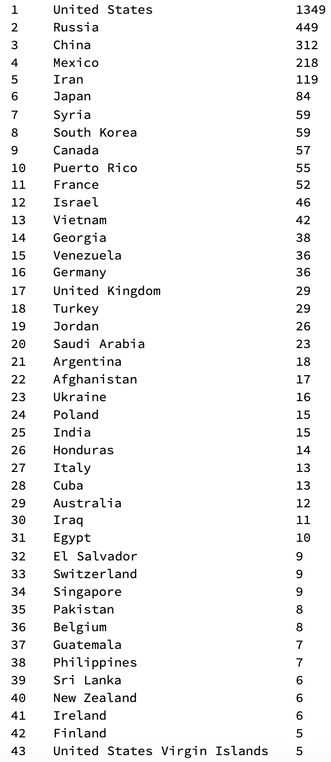
(This is only the top of the list.) Note, that North Korea is missing, but will be very prominent in the next table.... Next we can check for "indirect" mentions of a country, i.e. Louvre would lead to a mention of France etc. We will find many more entities and will first generate a list of substitution rules:
countriesrules = # -> Check[GeoIdentify["Country", #], {#}] & /@ (Complement[DeleteDuplicates[locations], EntityList[EntityClass["Country", "Countries"]]]);
We will ignore the error messages for now. We can then generate a table that includes the "indirect" mentions, too:
TableForm[Flatten /@ Transpose[{Range[Length[#] - 1], Delete[#, 5]}] &@({#[[1]], #[[2]]} & /@
 Normal[ReverseSort[Counts[CommonName@(DeleteMissing[Flatten[locations /. countriesrules]])]]])]
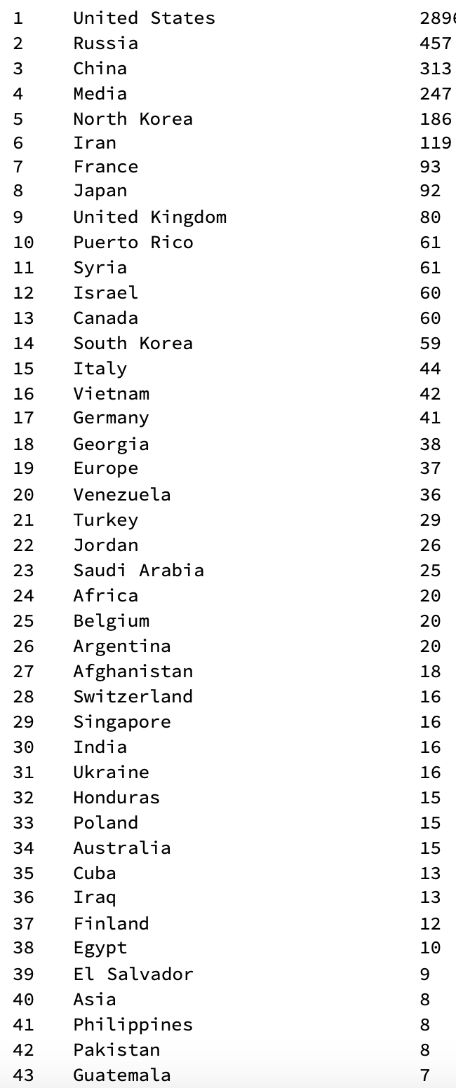
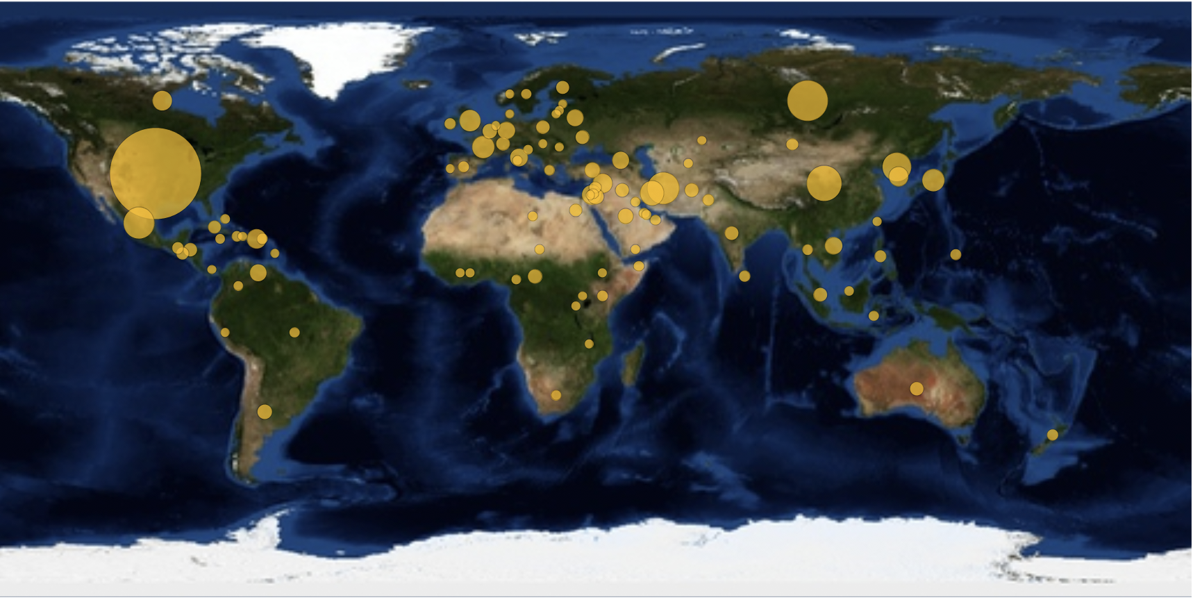
Note, that on rank 4 we find Media, which is not a country. It is easy to clean out, but I leave it in to show the performance of the code so far. We could now make typical representations such as GeoBubbleCharts:
GeoBubbleChart[Counts[DeleteMissing[Flatten[locations /. countriesrules]]], GeoBackground -> "Satellite"]
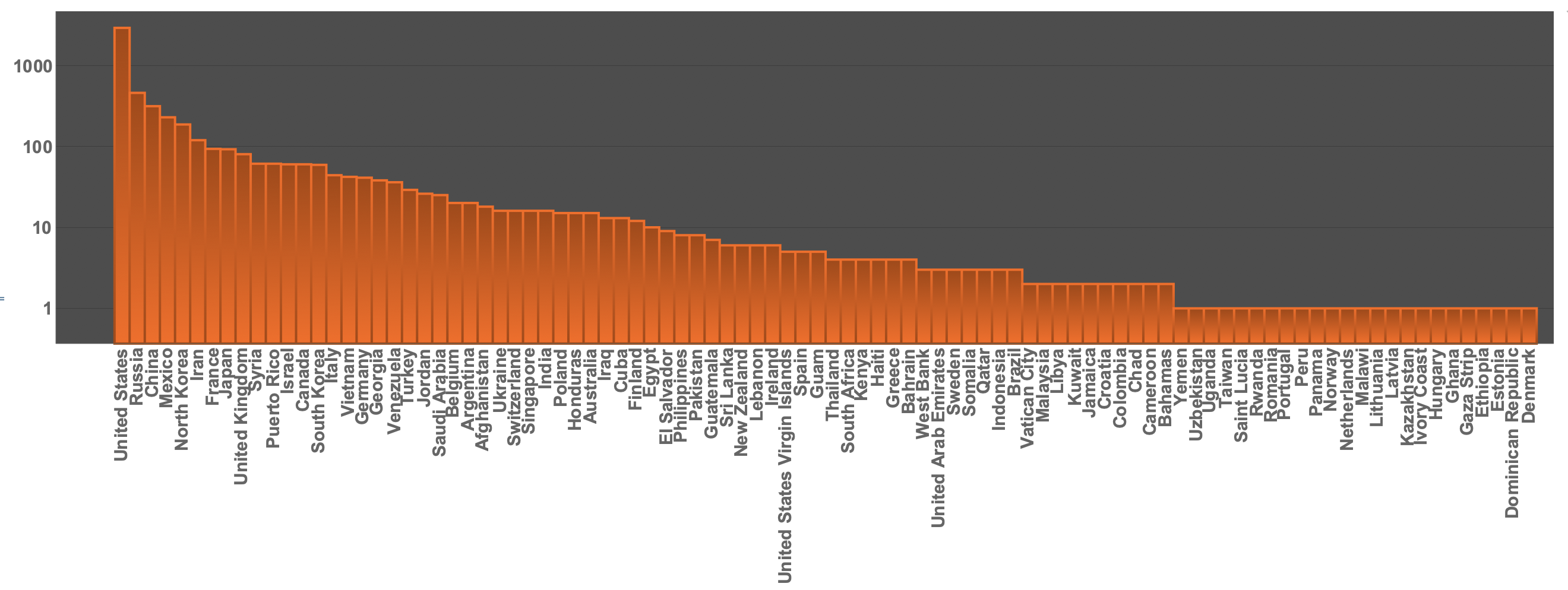
We can now make a BarChart (on a logarithmic scale) selecting "purecountries" like so:
BarChart[ReverseSort@<|
   Select[Normal@
     Counts[DeleteMissing[Flatten[locations /. countriesrules]]],
    MemberQ[purecountries[[All, 1]], #[[1]]] &]|>,
 ScalingFunctions -> "Log",
 ChartLabels -> (Rotate[#, Pi/2] & /@
    CommonName[
     ReverseSortBy[
       Select[Normal@
         Counts[DeleteMissing[Flatten[locations /. countriesrules]]],
        MemberQ[purecountries[[All, 1]], #[[1]]] &], Last][[All,
       1]]]), PlotTheme -> "Marketing",
 LabelStyle -> Directive[Bold, 15]]
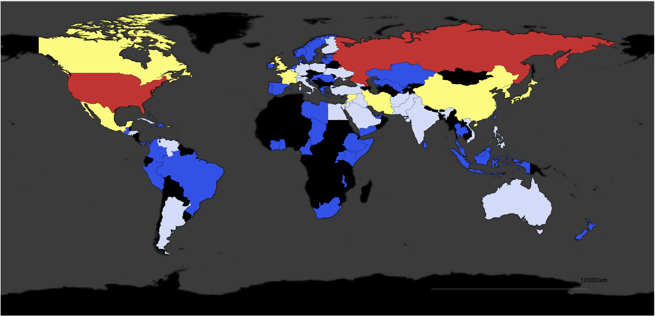
We can also represent that on a world wide map:
styling = {GeoBackground -> GeoStyling["StreetMapNoLabels",
GeoStylingImageFunction -> (ImageAdjust@ColorNegate@ColorConvert[#1, "Grayscale"] &)],
GeoScaleBar -> Placed[{"Metric", "Imperial"}, {Right, Bottom}], GeoRangePadding -> Full, ImageSize -> Large};

GeoRegionValuePlot[
Log@<|Select[Normal@Counts[DeleteMissing[Flatten[locations /. countriesrules]]], MemberQ[purecountries[[All, 1]], #[[1]]] &]|>, Join[styling, {ColorFunction -> "TemperatureMap"}]]
Further analysis
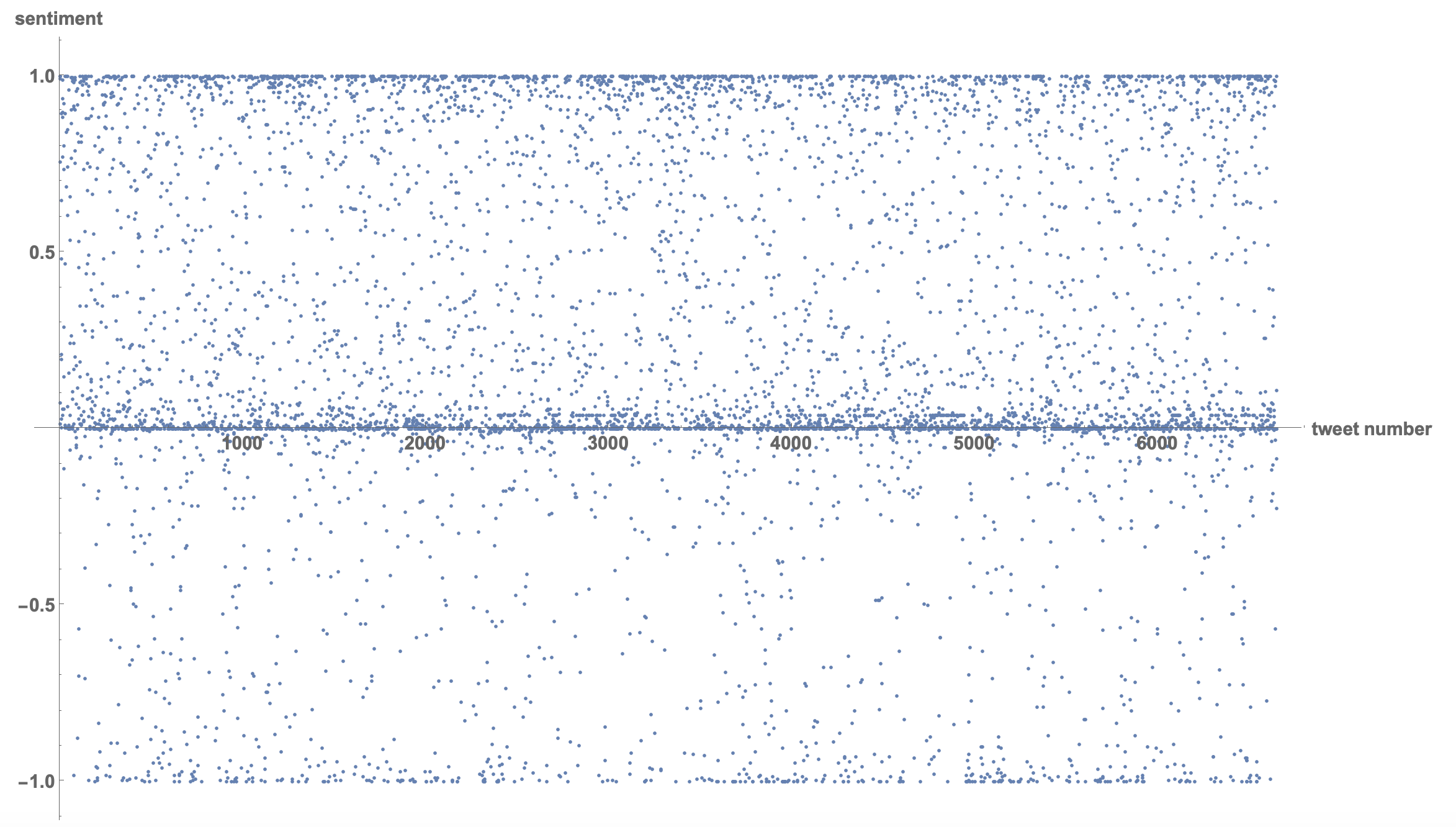
We can of course look at many other features of the tweets. One is a simple sentiment analysis. I am not at all convinced that the result of this attempt are useful or representing an actual pattern. But this is what we could do:
emotion[text_] := "Positive" - "Negative" /. Classify["Sentiment", text, "Probabilities"]
and then
tweetssentiments = emotion /@ tweettexts;
ListPlot[tweetssentiments, PlotRange -> All, LabelStyle ->
 Directive[Bold, 15], AxesLabel -> {"tweet number", "sentiment"}]
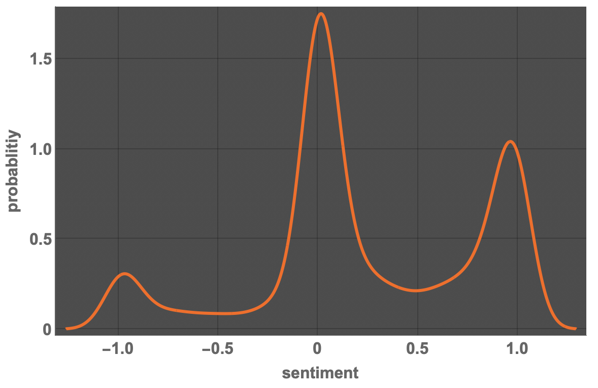
Using a SmoothHistogram, we see a pattern of "extremes", negative, neutral, positive:
SmoothHistogram[tweetssentiments, PlotTheme -> "Marketing",
 FrameLabel -> {"sentiment", "probablitiy"},
 LabelStyle -> Directive[Bold, 16], ImageSize -> Large]
We can also ask for less relevant information, such as the colours mentioned in the tweets:
textcasesColor = TextCases[StringJoin[tweettexts], "Color" -> "Interpretation", VerifyInterpretation -> True]

So there is a lot of white, some black, red and green:
ReverseSort@Counts[textcasesColor]

Let's blend these colours together:
Graphics[{Blend[textcasesColor], Disk[]}]

We can also look for "profanity" in tweets:
textcasesProfanity = TextCases[StringJoin[tweettexts], "Profanity"];
and represent these tweets in a table:
Column[textcasesProfanity, Frame -> All]
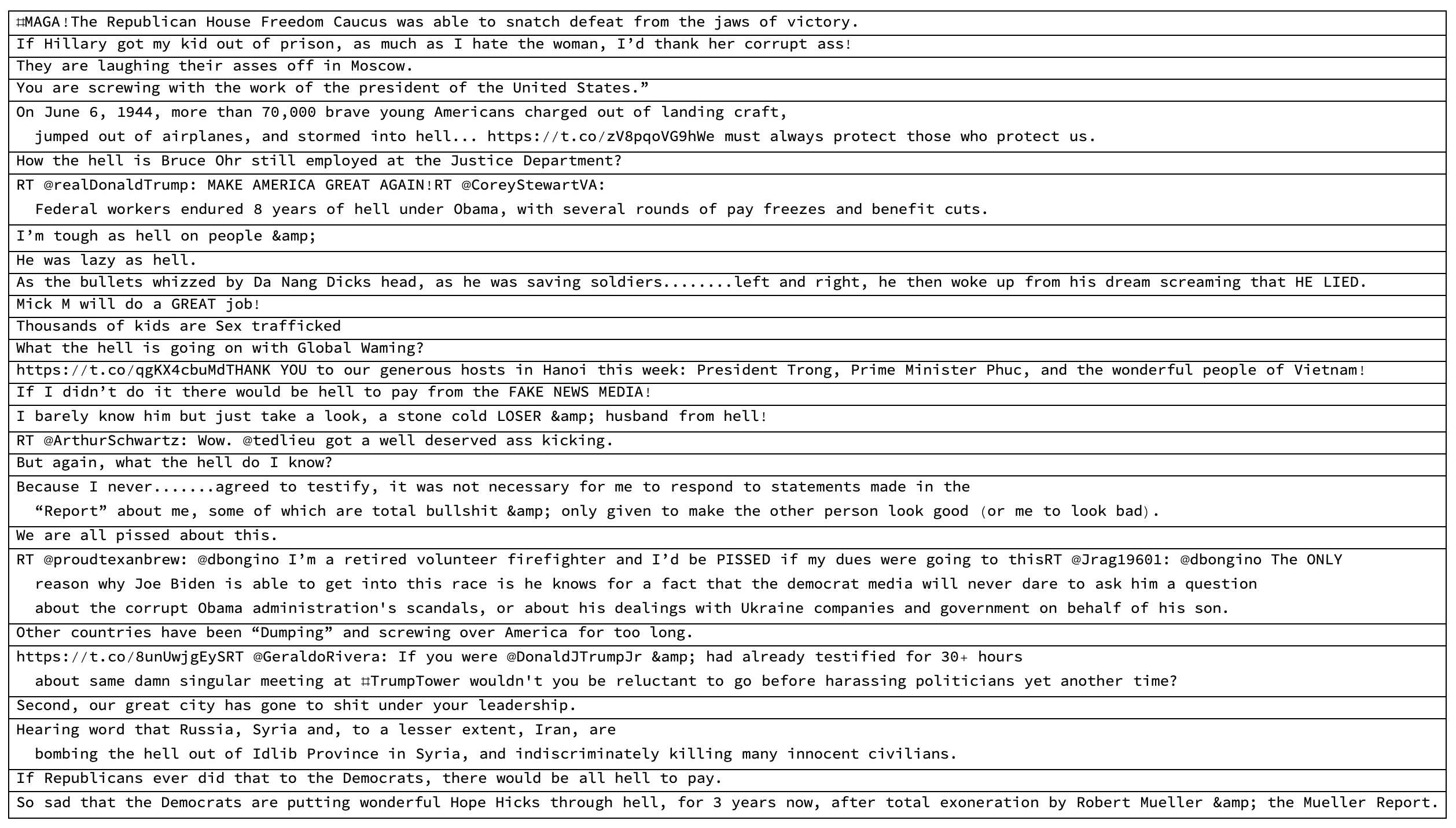
It is not quite clear to my why some of the tweets are classified as containing profanity. For some tweets it is relatively obvious, I think.
Twitter handles
Another interesting analysis is to look at the twitter handles that @realDonaldTrump uses:
textcasesTwitterHandle = TextCases[StringJoin[tweettexts], "TwitterHandle"];
Here are counts of the 50 most common handles:
twitterhandles50 = Normal[(ReverseSort@Counts[ToLowerCase /@ textcasesTwitterHandle])[[1 ;; 50]]]

Last but not least we can make a BarChart of that:
BarChart[<|twitterhandles50|>, ChartLabels -> (Rotate[#, Pi/2] & /@ twitterhandles50[[All, 1]]),
LabelStyle -> Directive[Bold, 14]]
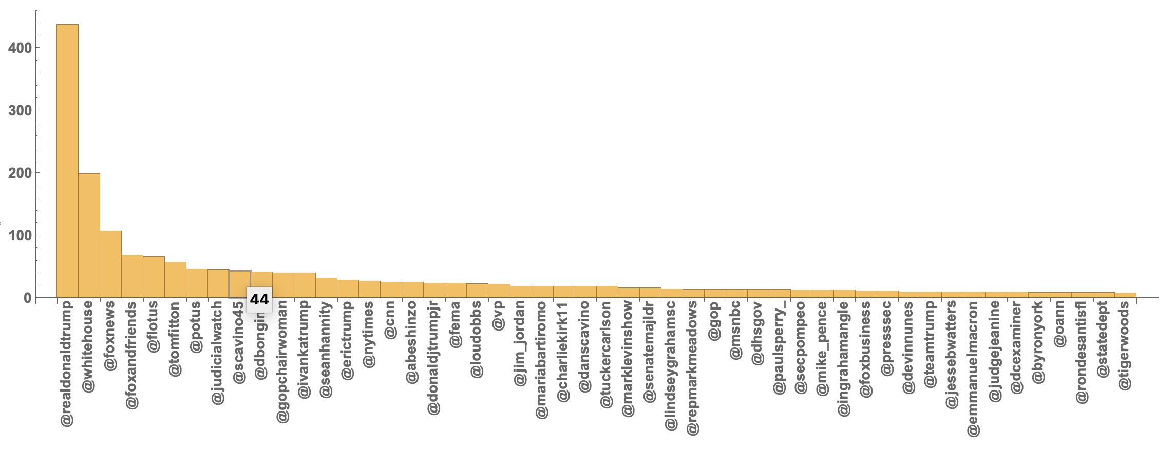
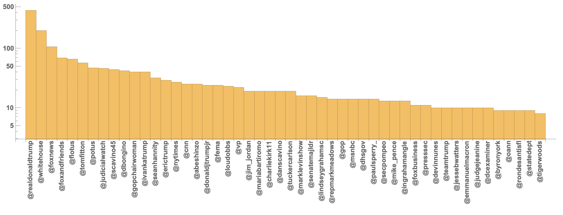
and to compare the same on a logarithmic scale:
BarChart[<|twitterhandles50|>, ChartLabels -> (Rotate[#, Pi/2] & /@ twitterhandles50[[All, 1]]),
LabelStyle -> Directive[Bold, 14], ScalingFunctions -> "Log"]
A little word cloud
Just to finish off we will generate a little word cloud like so:
allwords = Flatten[TextWords /@ tweettexts];
WordCloud[ToLowerCase /@ DeleteCases[DeleteStopwords[ToString /@ allwords], "&"]]
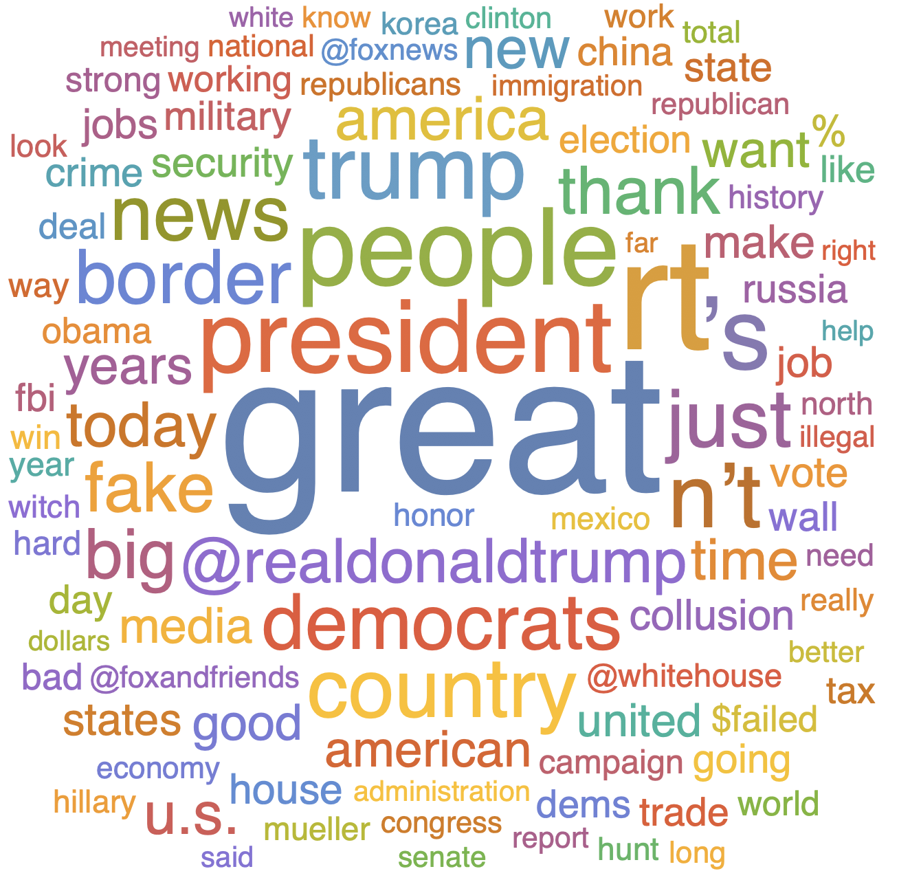
The cloud picks up on "witch hunt" and "collusion", "@foxandfrieds" and "Russia", "fake", "border" as well as other terms that indeed are relatively prominent in the media.
Conclusion
The main objective of this was to look try to reproduce at least qualitatively the results of the twitter analysis of @realDonaldTrump's tweets by The Economist using the Wolfram Language. We have been using a slightly different period of the tweets. We have been looking at direct mentions and "indirect" ones. I have not made any manual comparison of the results. I am not sure whether the recognition has worked and I only post it as a first cursory analysis.
It was relatively easy to go beyond the analysis and look at other features of the tweets, too.
 Attachments: