Abstract

The goal of this project was to simulate binary star systems and demonstrate the process of finding binary star systems and their populating planets. To accomplish this goal, I used a function called NBodySimulation, which describes the motions of a number of bodies subjected to predefined laws of motion. Simulating binary star systems, I produced a number of animations that describe the motions of these celestial bodies visually. After I succeeded in creating these animations, I moved to illustrate a practice called photometry, which astronomers use to detect binary star systems and exoplanets. I, following in the footsteps of these astronomers, produced a series of graphics describing the change in a binary star system's brightness over time.

Introduction

In 1929, Edwin Hubble discovered the Andromeda galaxy and destroyed our preexisting perceptions of the universe. The size of the universe expanded from 100 thousand light years across to 100 billion. The probability that there exists a planet that is similar to our own increases with every galaxy that is discovered. What was once a fantasy has become a near-reality. Consequently, the search for binary star systems and their populating planets has gained a great deal of attention. Astronomers everywhere are feverishly searching for binary star systems and their populating planets. Unfortunately, finding exoplanets is an incredibly difficult task, so dim and distant are they. Astronomers use photometry—the art of measuring changes in the intensity of light emitting from a defined area—to detect these celestial bodies. In this project, I demonstrate how astronomers detect binary star systems and their planets using photometry.

Simulating Binary Star Systems

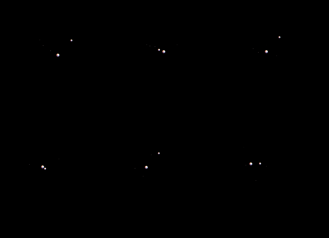
Here, I have created a simulation of a complete planetary system populated with a binary star and five planets.

ExoDataF = 
  NBodySimulation[
   "Newtonian", {<|"Mass" -> SM1, "Position" -> SP1, 
     "Velocity" -> SV1|>,
    <|"Mass" -> SM2, "Position" -> SP2, "Velocity" -> SV2|>,
    <|"Mass" -> PM1, "Position" -> PP1, "Velocity" -> PV1|>,
    <|"Mass" -> PM2, "Position" -> PP2, "Velocity" -> PV2|>,
    <|"Mass" -> PM3, "Position" -> PP3, "Velocity" -> PV3|>,
    <|"Mass" -> PM4, "Position" -> PP4, "Velocity" -> PV4|>,
    <|"Mass" -> PM5, "Position" -> PP5, "Velocity" -> PV5|>}, 
   Quantity[10^30, "Years"]];

Manipulate[
 Graphics3D[{White,
   Sphere[Values[ExoDataF["Position", t]][[1]], p*SR1],
   Sphere[Values[ExoDataF["Position", t]][[2]], p*SR2], Gray,
   Sphere[Values[ExoDataF["Position", t]][[3]], 2 p*PR1],
   Sphere[Values[ExoDataF["Position", t]][[4]], 2 p*PR2],
   Sphere[Values[ExoDataF["Position", t]][[5]], 2 p*PR3],
   Sphere[Values[ExoDataF["Position", t]][[6]], 2 p*PR4],
   Sphere[Values[ExoDataF["Position", t]][[7]], 2 p*PR5]}, 
  Background -> Black, Boxed -> False, 
  PlotRange -> {{-2*^12, 2*^12}, {-2*^12, 2*^12}, {-2*^12, 2*^12}}],
 {p, 10^5, 10^6},
 {t, 0, ExoDataF["SimulationTime"]/4, 1},
 SaveDefinitions -> True]

To create this simulation, I pulled data from the Alpha Centauri system to generate the stars and data from our solar system to generate the planets. This simulation is not representative of an actual binary star system; it has been artificially generated. With that said, it can be used to demonstrate the difficult nature of detecting exoplanets. It is relatively easy to detect the two stars (represented as large, white spheres); however, it is much more difficult to detect their populating planets (represented as small, gray spheres). Despite access to state-of-the-art equipment, astronomers also struggle to detect exoplanets. They have to resort to other methods.

Using Photometry to Detect Exoplanets

One can detect binary star systems and exoplanets by plotting the intensity of the light that an area in space is emitting vs time. Here, I plot the intensity of the light that a single star in space that is unpopulated with planets is emitting vs time.

ImageA =
  Table[
   ImageResize[#, {75, 75}]
     & /@ (Binarize[Graphics3D[{
        Glow[White], Black, Sphere[{0, 0, 0}, 500000 SR1]},
       Background -> Black, Boxed -> False,
       PlotRange -> {{-3*^12, 3*^12}, {-3*^12, 3*^12}, {-3*^12, 
          3*^12}}]]), 40];

ImageAData = ImageData /@ ImageA;

ListLinePlot[Count[1] /@ (Flatten /@ ImageAData), 
 PlotLabel -> "Brightness Curve", AxesLabel -> {"Time", "Brightness"}]

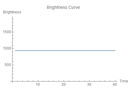
Unsurprisingly, the intensity of the light does not fluctuate over time. From this graph, one determines that there exists exactly one star and zero planets in this area.

Here, I plot the intensity of the light that a binary star system emits over time.

ImageB =
  Take[
   Flatten[
    Table[ImageResize[#, {75, 75}]
       & /@ (Binarize[Graphics3D[{
          Glow[White], Black, 
          Sphere[Values[ExoDataF["Position", t]][[1]], p*SR1],
          Sphere[Values[ExoDataF["Position", t]][[2]], p*SR2]},
         Background -> Black, Boxed -> False,
         PlotRange -> {{-3*^12, 3*^12}, {-3*^12, 3*^12}, {-3*^12, 
            3*^12}}]]),
     {p, {500000}},
     {t, 0, ExoDataF["SimulationTime"]/2, 
      ExoDataF["SimulationTime"]/100}]], 40];

ImageBData = ImageData /@ ImageB;

ListLinePlot[{Count[1] /@ (Flatten /@ ImageBData)}, PlotRange -> All, 
 PlotLabel -> "Brightness Curve", AxesLabel -> {"Time", "Brightness"}]

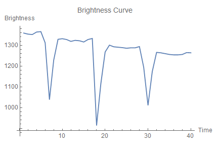
Notice that the intensity of the light dips periodically. These fluctuations indicate that there exist two celestial bodies.

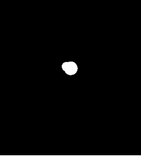
The intensity of the light is greatest when both bodies are visible:

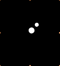
And least when one body eclipses the other:

Here, I plot the intensity of the light that a binary star system populated with exactly one planet emits.

ImageC =
  Take[
   Flatten[
    Table[ImageResize[#, {75, 75}]
       & /@ (Binarize[Graphics3D[{
          Glow[White], Black, 
          Sphere[Values[ExoDataF["Position", t]][[1]], p*SR1],
          Sphere[Values[ExoDataF["Position", t]][[2]], p*SR2],
          Glow[Black], 
          Sphere[Values[ExoDataF["Position", t]][[4]], 3 p*PR2]},
         Background -> Black, Boxed -> False,
         PlotRange -> {{-3*^12, 3*^12}, {-3*^12, 3*^12}, {-3*^12, 
            3*^12}}]]),
     {p, {500000}},
     {t, 0, ExoDataF["SimulationTime"]/2, 
      ExoDataF["SimulationTime"]/100}]], 40];

ImageCData = ImageData /@ ImageC;

ListLinePlot[{Count[1] /@ (Flatten /@ ImageCData)}, PlotRange -> All, 
 PlotLabel -> "Brightness Curve", AxesLabel -> {"Time", "Brightness"}]

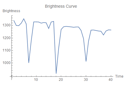
One determines that there exist two stars and at least one planet by observing the magnitude of each fluctuation. A change of 200 units indicates that one of the stars eclipses the other. A change of 30 units a planet. The planet is much smaller than both of the two stars; therefore, it has a much smaller impact on the intensity of the light emitting from the area.

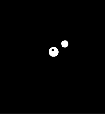
Notice that the planet covers but a small portion of the stars:

Conclusions

It is difficult to detect binary star systems and their populating planets; however, it is not impossible. Using photometry, astronomers can uncover small, dimly-lit bodies orbiting stars light years away. In this project, I explain how difficult it is to detect the planets populating a binary star system and demonstrate the methods used to do so. I had to learn how to use a function called NBodySimulation in order to produce the simulations shown in this notebook. Once I learned how to use this function effectively, I began generating data and creating visualizations depicting dots in a 2D plane. Most of the simulations that I created I made using data that I generated. After producing these simulations, I moved to create a complete planetary system populated with a binary star and five planets. Generating this simulation, I noticed that the planets are difficult to see, much smaller and dimmer than their parents. I began to wonder how astronomers detect binary star systems and their populating planets, which led me to investigate a practice used to detect these bodies called photometry. To demonstrate how one detects binary star systems and exoplanets using photometry, I produced a series of graphs that depict the changes in the intensity of the light emitting from the window. One should be able to detect the stars and planets in the simulation solely from these graphs.

Future Works

Allotted more time, I would design a function that would allow the user to alter the masses, radii, positions, velocities, and number of bodies present in the interface in real time. I attempted to apply Manipulate to NBodySimulation, but since NBodySimulation produces cooked data, such an approach is not applicable. I also would create a visualization describing what happens when a star expands beyond its Roche Lobe. Such a visualization would help illustrate the chaotic nature of these binary star systems. I also would produce a visualization depicting what one would see, standing on the surface of an exoplanet looking up. Imagine standing on the surface of a planet orbiting between a pair of stars. Everywhere is day; only along the planets prime meridian would you be able to experience twilight. It would have been a fun, engaging endeavor to try to create such a visualization.

Definitions

I generated the data to make the simulations shown here. However, I based these numbers on data that I pulled on the Alpha Centauri system and the planets present in our solar system.

SM1 = Quantity[2.188*^32, "kg"];
SM2 = Quantity[2.80402*^31, "kg"];
PM1 = Quantity[2.00*^24, "kg"];
PM2 = Quantity[1.97*^26, "kg"];
PM3 = Quantity[3.35*^23, "kg"];
PM4 = Quantity[5.69*^24, "kg"];
PM5 = Quantity[2.777*^25, "kg"];

SR1 := 8.511*^5;
SR2 := 6.005*^5;
PR1 := 6.371*^4;
PR2 := 6.991*^4;
PR3 := 2.439*^4;
PR4 := 6.371*^4;
PR5 := 5.823*^4;

SP1 = Quantity[{0, 0, 0}, "AstronomicalUnit"];
SP2 = Quantity[{0, 11.2, 0}, "AstronomicalUnit"];
PP1 = Quantity[{-11.2, 5.6, 0}, "AstronomicalUnit"];
PP2 = Quantity[{0, -5.2, 5.2}, "AstronomicalUnit"];
PP3 = Quantity[{5.2, -5.2, 13.5}, "AstronomicalUnit"];
PP4 = Quantity[{1, -11.2, 11.2}, "AstronomicalUnit"];
PP5 = Quantity[{1, 13.5, -5}, "AstronomicalUnit"];

SV1 = Quantity[{-21.4, 0, 0}, "km"]/sec;
SV2 = Quantity[{20.6, 0, 0}, "km"]/sec;
PV1 = Quantity[{20.5, 0, 0}, "km"]/sec;
PV2 = Quantity[{0, 15.7, 0}, "km"]/sec;
PV3 = Quantity[{-19.5, 0, 0}, "km"]/sec;
PV4 = Quantity[{-21.5, 0, 0}, "km"]/sec;
PV5 = Quantity[{0, 18.9, 0}, "km"]/sec;

References

“Transit Photometry: A Method for Finding Earths.” The Planetary Society, www.planetary.org/explore/space-topics/exoplanets/transit-photometry.html. Accessed 11 Jul. 2019.

“Discovery: Other Galaxies Exist.” Amazing Space, amazing-space.stsci.edu/resources/explorations/groundup/lesson/scopes/mt_wilson/discovery.php. Accessed 11 Jul. 2019.