Mountains have a huge impact on weather and climate conditions and are important landmarks. The aim of my project was to classify the position of a mountain using its elevation data as an input.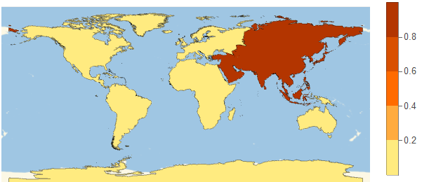

Project Description

My final program classifies the country of a given mountain using its elevation data as an input. The data is sent to a neural network, which was trained on the elevation data of the five highest mountains per country in Europe. Then, the program returns a map displaying the location of the mountains.

Another neural network, trained on the ReliefPlot of the ten highest mountains per continent, identifies the continent to which the elevation data belong and then plots the probabilities of a mountain belonging to the continents using a map with different colors. However, this method is more time consuming because of the data size.

The third approach is to recognize a mountain by its profile which you can easily create by using the ListPlot3D function.

Overview

To implement this project, I had three different approaches, of which one turned out to be the most efficient one. I started by 3D-Plotting the ten highest mountains in the world, editing the plot and then fitting pictures from different viewpoints of the mountains to a neural network. Thereby, the mountains are identified by their profile. In order to train a useful neural network, a great amount of data is required. This means that you have to create many slightly different pictures by changing the GeoRange, which is the length of the shown part, and the viewpoints, which are the angles from where you look at the mountains. This method did not turn out to be useful, because the performance of my computer could not compete with the requirements in terms of required number of graphics in a reasonable amount of time.

Another way to accomplish the project was to train a neural network by using the surface plots of the mountains. I trained the network on the ten highest mountains of each continent. To create more data, I changed the GeoRange and the center of the plot to up to 100 feet to the east. The respective result is promising. By using GeoElevationData as input data, the program returns the respective probabilities for the continents, which are then illustrated on a map. However, similar to the first approach, memory problems of my computer occurred when creating more data and considering the 5 highest mountains for each country.

The simplest way to handle the problem is to use only the GeoElevationData. In my third approach, I implemented this strategy by specializing on the five highest mountains of all countries in Europe. Therefore, I created data, which were varied by different GeoRanges, by shifting the center of the graphic up to 100 meters to the east.

1) Identifying a mountain by its profile

Part of my approach was to identify a mountain by its 3D plot. This works by using the ListPlot3D function. An example picture of the Mount Everest is given here:

ListPlot3D[
  Reverse[GeoElevationData[Entity["Mountain", "MountEverest"], 
    GeoRange -> Quantity[10, "Kilometers"], 
    GeoProjection -> Automatic]], ViewPoint -> Front, Axes -> False, 
  Mesh -> None, BoundaryStyle -> None, Boxed -> False, 
  ImageSize -> Medium] // Rasterize 

As a result, you can see this 3D-plot:

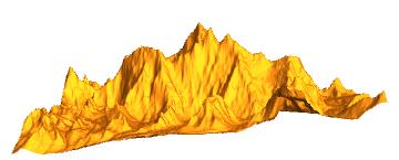
To create a meaningful dataset, I rasterized plots of the 10 highest mountains in the world. To get slightly different pictures, I varied the GeoRange and the ViewPoint. I also set the PlotStyle on black, changed the lighting and filled the bottom black.

There will be 41 * 5 * 4 = 820 different images for each mountain. That means that there will be 820 * 10 = 8200 images in total. This is a good size to train the model.

In order to prevent that a new plot is created whenever the GeoElevationData is downloaded, I created a function, which saves the elevation and just changes the viewpoint.

plotDatasetTenHighestMountains [mountain_, range_]:= 
    (plot = 
       ListPlot3D[
         Reverse[
          GeoElevationData[
              mountain, GeoRange->Quantity[
                 range, "Kilometers"
              ], GeoProjection->Automatic]
          ], Mesh->None, ImageSize->{224, 224}, Boxed->False, Axes->False, BoundaryStyle->None, PlotStyle->Black, Lighting->{"Ambient", White}, Filling->Bottom, FillingStyle->Black]; 
       Table[
         Rasterize@Show[
          plot, ViewPoint-> {2 Cos[theta], 2 Sin[theta], z}
         ], {theta, 0, 2 Pi, 1/20 Pi}, {z,0,0.7,0.2}
       ]
    )

Creating the data is not working in my case because of my computer's limited memory. Nevertheless, you can find an explanation how to carry on in my computational Essay.

Conclusion

Due to my limited computer memory, it was only possible to create a limited dataset with pictures containing plots of mountains.Therefore, the method, determining the position of the mountain via a classification of the mountain and then referring to the position of the mountain, was not applicable in my case.

2) Identifying a mountain by its ReliefPlot

Plotting the relief of a mountain

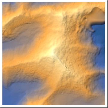
By using ReliefPlotFunction and a GeoRange of 4 kilometers, the relief can be plotted. The relief of the Mount Everest is shown as an example.

ReliefPlot[
    GeoElevationData[
       Entity["Mountain", "MountEverest"], GeoRange->Quantity[2,"Kilometers"], GeoProjection->Automatic
    ]
]

The result is the following plot:

For each continent, I created a dataset of the ReliefPlots of the 10 highest mountains.

DatasetMountainsInContinent =
    Table[
       ReliefPlot[
         GeoElevationData[
          mountainsInContinent[[m]], GeoRange-> Quantity[2, "Kilometers"], GeoProjection->Automatic], ImageSize->{224,224}], {m, 1, Length[mountainsInContinent]}];

To create more data, I changed the GeoRange from 1 km to 20 km in steps of 4 km and shifted the midpoint of the ReliefPlot from 20 ft to 100 ft in steps of 25 ft.

DatasetMountainsInContinentAdd = 
    Flatten[
       Table[
         ReliefPlot[
          GeoElevationData[
              GeoRange -> Quantity[x, "Kilometer"],GeoProjection->Automatic, GeoCenter-> GeoDestination[
                 (mountainsInContinent[[m]]["Position"]),{y,90}
              ]
          ]
         ],{m,1,Length[mountainsInContinent]},{y,20,100,25}, {x,1,20,4}
       ]
    ];

To train a Neural Network, the data needs to be labeled. To do that, I created a list of labels and then I created an Association between SurfacePlot and label which is then converted into a list.

For the first dataset, the labels are created by plotting the name of every continent in the order of the list continentsnames considering the length of the list DatasetMountainsInContinent and the number of continents how often the names are behind each other. This method assumes that each continent has the same number of mountains, which is the case.

For the second dataset, I copied the method, just that instead of the list DatasetMountainsInContinent, I took the list DatasetMountainsInContinent2.

Create a classifier

In order to best train the classifier, I scrambled the data to prevent patterns. I then split the dataset into trainingdata and testdata and trained a classifier with the trainingdata. I measured the performance of the trained classifier with the testingdata and plotted the ConfusionMatrix:

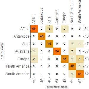
The accuracy is at about 0.95.

By using the following code, probabilities were plotted in a map:

GeoRegionValuePlot[
    Table[
       Entity[
         "GeographicRegion", StringReplace[
          ToString[
              Keys[
                 cContinent[
                   ReliefPlot[input], "Probabilities"
                 ]
              ][[y]]
          ], " "->""
         ]
       ]-> Values[
         cContinent[
          ReliefPlot[input], "Probabilities"
         ]
       ][[y]], {y, 1, Length[cContinent[ReliefPlot[input], "Probabilities"]]}
    ]
]

The input is from the user in form of a GeoElevationData, cContinent is the trained Classifier. For example, the map of Mount Everest's GeoElevationData is:

Conclusion

By using this approach, it is possible to determine the continent and mark it on a world map. To go into more detail and to be able to predict the country, I would require much more data. As you have already seen in the first approach, my computer does not have enough memory for creating many graphics.

3) Identifying the mountain's position by its elevation data

The goal is to classify the country by the elevation data of the 10 highest mountains of each country.

Thereby, I created a list of the GeoElevationData where each sublist belongs to a country (alphabetical order). Because there are not five mountains in each sublist (for instance Vatican City does not have any mountains) you cannot create the labels in the way I did before.

I first created an empty list for the labels and then considered the list of mountains in Europe. The elements of the same sublist belong to the same country, that means that they have the same label. Step by step, I looked at each sublist. In each sublist, I created as many labels for the countrys as there are elements in the sublist. It is important to know that the nth sublist belongs to the nth country. Some countries do not have any elements, so by counting the elements in the sublist and then by creating that many labels, it is possible that one country does not have any label. This is no problem though, because there is no element in the ElevationDataList.

Because of the high number of mountains, I did not want to download the GeoElevationData every time, but I just wanted to change the GeoCenter and the GeoRange from the unique downloaded GeoElevationData. In addition to that, the created GeoElevationData are saved into a directory. If there is already a file that is named in that way, the program will not create another one. In the case of a mountain that does not have GeoElevationData, I catch the error with the functions Quiet and Check with the parameter of an empty list {}. In addition to that, I monitor the current values of y, x and m to see how fast the program is running.

Block[{geo}, 
    Table[
       With[
         {filename = ToString@x<>"-"<>ToString[y]<>"-"<>ToString[m]<>".mx"},
         If[
          !FileExistsQ[filename], 
          geo = Quiet[
              Check[
                 GeoElevationData[
                   GeoRange -> Quantity[x, "Kilometer"],GeoProjection->Automatic, GeoCenter -> GeoDestination[(mountainsInEurope[[m]]["Position"]),{y,90}]
                 ],{}
              ]
          ];
         DumpSave[filename, geo]
         ]
       ];,{y,20,100,20}, {x,1,20,4},{m,1,Length[mountainsInEurope]}
    ]
]~Monitor~{y,x, m};

After that, a list is created of the GeoElevationData by taking the FileNames and adding them to the list. If you look at the AbsoluteTiming, you can see that this method is much faster than the earlier approches.

DatasetMountainsInEuropeAdd = 
    Block[
       {geo},Table[
         If[MatchQ[ToExpression/@StringSplit[FileBaseName[f], "-"], 
         {Alternatives@@Range[1,20,4], Alternatives@@Range[20,100,20], _}],
          Get[f]; geo,Nothing], {f, FileNames["*-*-*.mx"]}
       ]
    ]~Monitor~f; //AbsoluteTiming

In order to get the total dataset, I had to create labels in the same order. As mentioned above, you cannot create labels, because there is not an equal number of mountains per country. By creating the DatasetMountainsInEuropeAdd, I used the Table function with the last parameter of the mountain. That means that the order of the countrys occurs repeatedly. A copy of this repeated order corresponds to the order of the already created label list.

As a conclusion, I can create the new Labels, by looking at the number how often the order is repeated and then adding the previously created list.

Creating and Training the classifier

The Length of the dataset is 4550. I splitted it into two sets: the trainingdata and the testingdata by randomly selecting 2825 indices of the full dataset and by using them for the trainingdata. The other indicies were used as testdata. The indices are also referring to the Position of the label in the labellist.

The structure of a ElevationData of one mountain is a QuantityArray with the Unit Feet. By using the function QuantityMagnitude, I deleted the Units. On top of that, I rescaled the array, that means that every value is between 0 and 1 and I created an image out of it.

itrain = Image/@ Rescale[trainingset];

I trained the Classifier with:

cEurope = Classify[itrain -> trainingsetOutcome, PerformanceGoal->"Quality", Method->"RandomForest"]

Before I can use the testdata, I had to modify it. I deleted the unity, going on with clipping it to prevent errors and then I rescaled them and converted them into an image. This needed to be done, because the Neural Network was trained on this datatype.

itestset=Image/@Rescale[Clip[QuantityMagnitude[testset],MinMax[trainingset]],MinMax[trainingset]];

An Image, created in that way, looks like that:

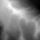(The changed QuantityArray of the Großglockner in Austria)

I now measuremented the Classifier with the itestset and looked at the ConfusionMatrix: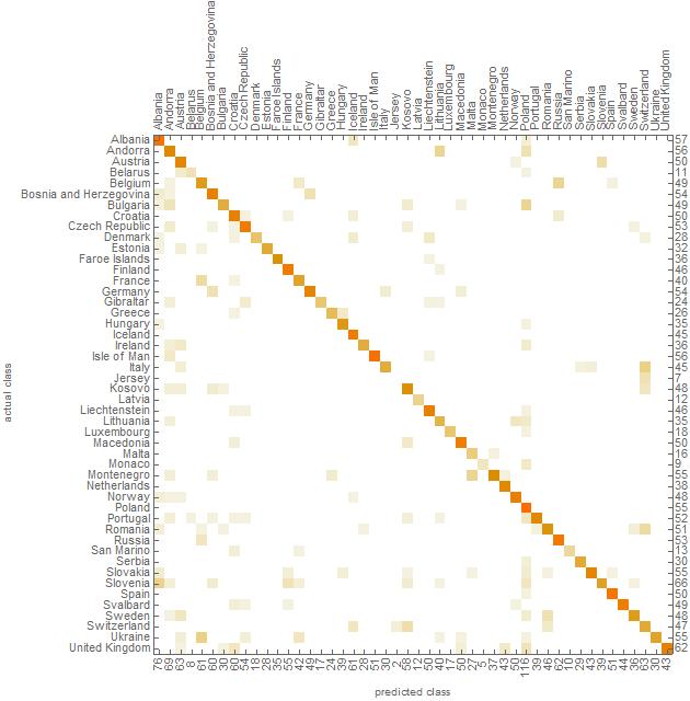

The accuracy is about 78.4% which is pretty good for the small ammount of data.

Visualization

The user can now Input a GeoElevationData, and the Input is changed to:

input = Image[Rescale[QuantityMagnitude[input]]]

The Input is sent to the Classifier and all the probabilities are then used as Input for the GeoRegionValuePlot function. One possible output would be: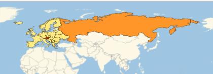

In this case, the country would be Austria

Future work

The Future Work can be roughly divided into 3 parts:

1. Create more data: do not just create more data for the same mountain, but for example: predictions for countries of other continents, more detailed description of the exact position, such as the city nearby
2. Improving the Neural Net: So far, only the Classify Function has been used. However, the functionality of a neural network can be improved by creating its own network or using transfer learning, e.g. with the “ResNet 101 Trained on YFCC100m Geotagged Data”. This model is already trained on the pictures of mountains, which could be related to the plots.
3. Add extra features. The user should not only get as a result in which continent / country / city a mountain is located, but also additional information such as height, degree of difficulty when climbing, best hiking trails...

Acknowledgements

I would like to thank my mentor, all the instructors at the Wolfram Summer Camp and every other person who made this camp unforgettable. They have been incredibly helpful and I have learned a lot of new things within these two weeks.