Please download the notebook attached at the end of this discussion

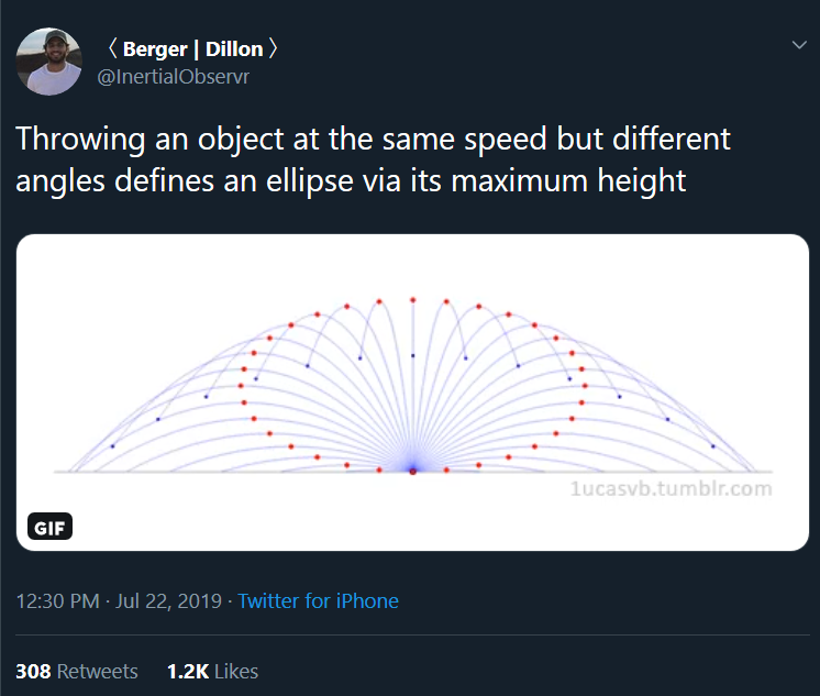
I found this twitter animation quite fascinating. Simple high school physics connects the conic section curves through a subtle way. Lets program this through Wolfram Language.
Assume initial throwing speed is $v_0 = 5$ meter per second:
v0 = 5;
and the gravity on earth is
g = QuantityMagnitude[Entity["Planet", "Earth"][EntityProperty["Planet", "Gravity"]], "Meters"/"Seconds"^2]
(* g = 9.80 meter per second sqaured*)
The kinetics and trajectory of a projectile are expressed in parametric form:
traj[\[Theta]0_, t_] := {v0*Cos[\[Theta]0]*t, v0*Sin[\[Theta]0]*t - (g*t^2)/2}
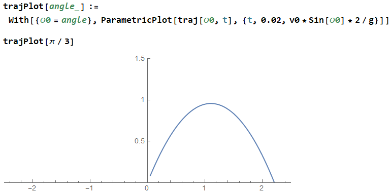
Given an angle that defines the throwing angle and ground, we can use the traj function to draw the corresponding trajectory:
trajPlot[angle_]:=With[{\[Theta]0=angle},ParametricPlot[traj[\[Theta]0,t],{t,0.02,v0*Sin[\[Theta]0]*2/g}]]

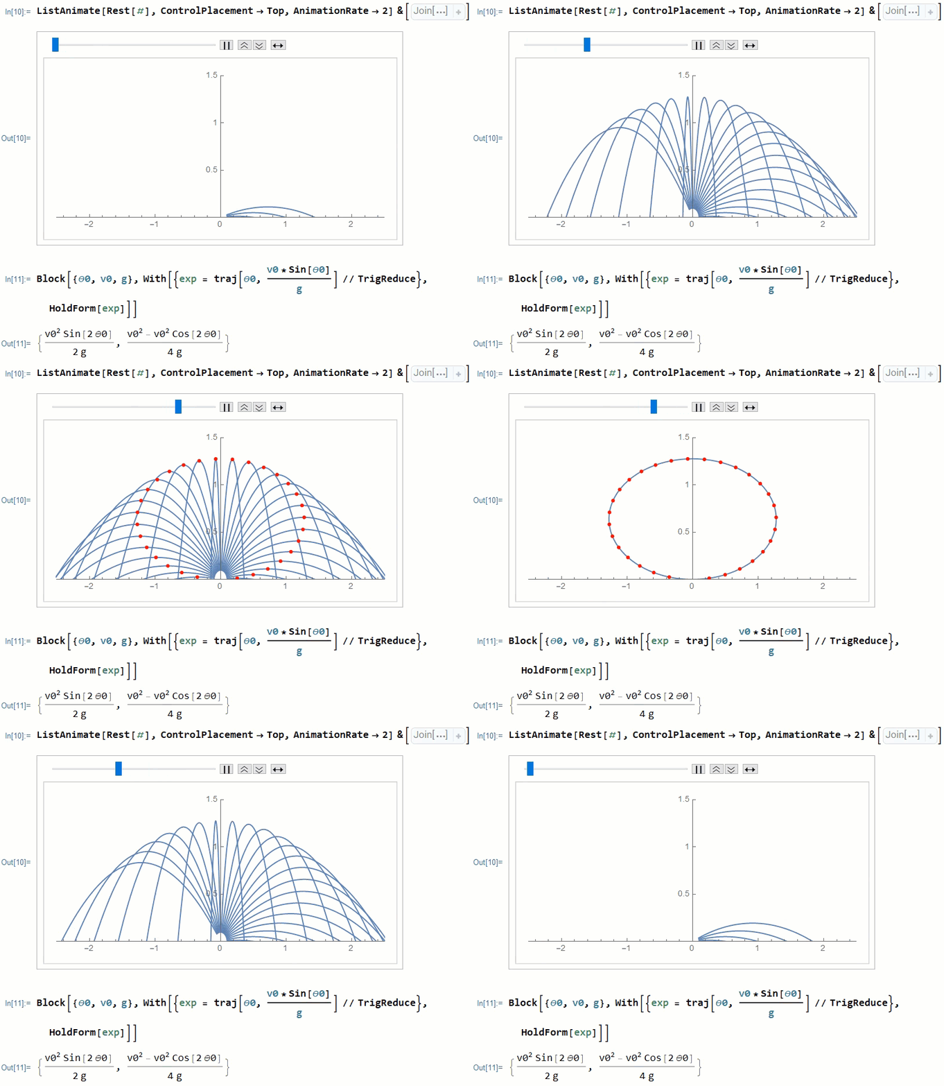
So in my animation that I am going to show later, all trajectory plot can be accumulated with FoldList and single frames which are generated in the above manner:
frames = Rest@FoldList[Show[#1, #2] &, Table[trajPlot[\[Theta]], {\[Theta], range}]];
Let's pick some throwing angles from $0$ to $\pi$: range = Range[0.1, \[Pi] - 0.1, 0.1];. Then all maximum heights can be computed directly because we know the ascending time stops when the vertical speed reduce to zero linearly due to gravity:
peaks = traj[#1, (v0 Sin[#1])/g] & /@ range;
Thus we can create a frame with all peak points through which define a ellipse passes.
peaksPlot=ParametricPlot[traj[\[Theta]0,(v0*Sin[\[Theta]0])/g],{\[Theta]0,0,\[Pi]},Epilog->Join[{Red,PointSize[Medium]},Point/@peaks]];
Now lets put peaksPlot and frames altogether in the ListAnimate function. The proof is also attached on the bottom of the animation. You can simply rearrange the terms in the Out[11] and use $\sin^2(2\theta) + \cos^2(2\theta) = 1$ to find the standard form of ellipse. This is left to our readers as homework.

 Attachments: